Information
Authors: V. Nemkov, V. Bukanin, A. Zenkov, A. Ivanov
Location/Venue: MEP 14 Hannover, Germany
Topic: Simulation of Slabs
Abstract
Presentation is devoted to simulation of slab heating in the longitudinal magnetic field. There were many studies of this technology in the past, but they were mainly related to heating materials with linear properties. One of the problems in slab heating simulation is a 3D character of the electromagnetic (EM) and thermal (T) processes. New program ELTA 6.0 has an option of 2D FDM simulation of EM and T processes in combination with semi-analytical account for the finite length of the system. Presentation contains a short survey of history and state-of-art of slab heating. New simulation procedure and a study of the edge effect variation during high temperature heating of the magnetic slab are presented. Example of simulation for multi-stage heating of big steel slab illustrates the theoretical considerations.
Introduction
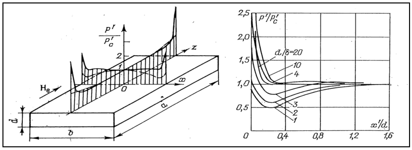
Heating of slabs was a subject of multiple studies since the beginning of 1960s [1]. We can mention here a work of V. Peysakhovich [2], who derived equations in the form of series for the field and power density distributions as well as for an impedance of a body with rectangular cross-section placed in the longitudinal magnetic field. The following studies of slab heating in 1970s were devoted to calculation of electromagnetic and thermal fields using analytical and later numerical Finite Difference Methods (FDM). An interesting study of the electrodynamic forces and methods of design of vibroresistant inductors for slab heating was published by L. Zimin in 1973 [3]. Multiple results of study of slab heating using analytical and numerical methods were conducted in LETI in 1970-1980s and published in a monograph [4]. Main attention was paid to power distribution and graphs for impedances which were presented for the non-magnetic and magnetic slabs in a wide range of skin effects and aspect ratios. It was shown that maximum efficiency in heating wide slabs corresponds to a ratio of slab thickness d and penetration depth δ equal to π. It is interesting that approximately the same ratio of d/δ provides the most uniform (in sense of uniformity “in large”) distribution of power in the width of the wide non-magnetic slab (see Fig. 1). It means that the this level of skin effect provides the most effective, fast and uniform heating of wide slab under adiabatic conditions. Changing frequency and therefore d/δ, one can provide required temperature distribution, e.g. for compensation of additional thermal losses from the slab sides. For selected frequency it is possible to design the coil providing required temperature distribution in the slab length by means of control of the End effects of the slab and coil (see Fig. 1).
Our experience shows that the terms “End effects” and “Edge effects” are not being used by different authors in the same way and it is worth to give clear definitions.
Edge Effects describe distortion of the electromagnetic field, current and power distributions caused by abrupt change in geometry or material properties in the eddy current flow path, e.g. near the edges of a slabor strip. Edge effects are especially important in the transverse heating of plates and strips.
Edge and End effects are typically two-dimensional and may be relatively easy studied and described using 2D simulation. The problem of simulation of slab heating is actually 3D and at the corner in the slab end plains we have the areas where Edge and End effects interfere. An example of current distribution in 3D area is presented in Chapter I of the Induction Training Course on a site http://fluxtrol.com/technical-library/induction-heating-training.
Surface power density p' is very convenient for description of end and edge effects (Fig. 1). Value of p' is an integral of volumetric power density pv along the slab thickness d. End effects are not considered in present paper due to limited space. Existing theoretical studies of slab heating are mainly related to materials with linear properties. For real cases of heating steel slabs, the skin effect can vary dramatically in the process of heating influencing both end and edge effects. In addition to that, the results of previous studies of edge effects are applicable accurately only to the slabs with aspect ratio b/d exceeding 4 otherwise the edge effects can interfere and influence both the coil parameters and power distribution.
1. Simulation of slab heating using ELTA 6.0
Program ELTA 6.0 is a new version of the industrial user-oriented program. It contains multiple improvements compared to the previous versions of ELTA with a completely new option for the induction heating of bodies with rectangular cross-sections (rods, billets, slabs, etc.). This option is based on a special 2D FDM algorithm for calculation of the coupled electromagnetic and thermal fields. It allows the user to investigate both power density and temperature distribution in the cross-section of the body during the whole process of heating. An analytical “Total Flux Method” is used for an account of a finite length of the coil and workpiece in the same way as in the previous versions. Total Flux method is based on composing the magnetic substitution circuit for a system “inductor–workpiece” [4]. Multiple tests show that it gives good practical results in simulation of 2D systems of simple geometry. In some cases even 3D systems such as heating of slabs in oval or rectangular inductors can be simulated with good accuracy [5].
ELTA 6.0 can simulate slab heating with 1D and 2D approaches. In both cases the system has two planes of symmetry OX and OY and simulation is being performed for a quarter of the cross-section. In 1D option the program calculates field strength, current and temperature versus the slab thickness in its central zone. This approach gives good results in temperature distribution only for a central zone and correct coil parameters for rather wide slab (b/d>8). One-dimensional calculation is also used at the beginning of each 2D simulation for two reasons: a) to provide good initial calculation setup for 2D calculation; b) to give the user fast reasonable answer regarding selected processing parameters (frequency, power, time, etc.) before accounting for edge effects. When using 2D option, the user can calculate and visualize the following additional items:
- Color maps of temperature, heat sources (power density) and magnetic field strength in the whole slab cross-section for any instant of heating –T,w,H = f(x,y @ any t).
- Color maps of temperature variation –T = f(x,t @ any y) and T = f(y,t @ any x).
- It is possible to change scale range of presented values for all color maps using Scale button); it make possible to display maps of absolute temperatures and of temperature gradients.
- Curves of temperature, heat sources and field strength along horizontal or vertical centerlines for any time instant T,w,H = f(x @y = 0 or y @ x = 0).
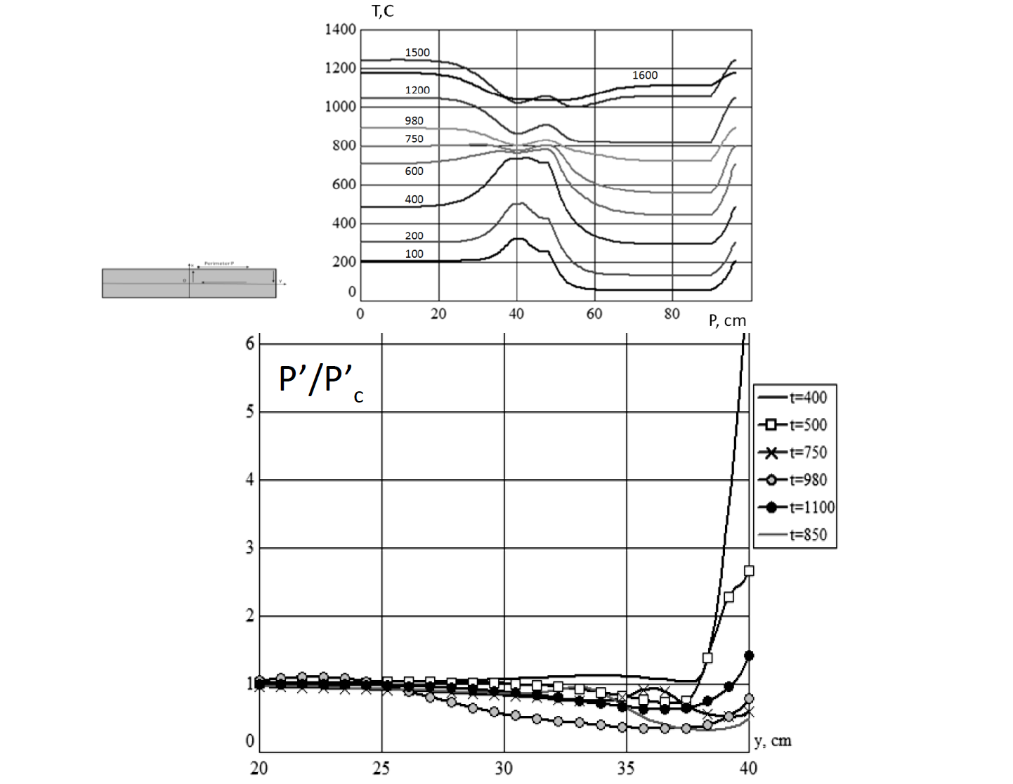
- Curves of temperature along the perimeter of one quarter of the slab, fig. 2, for any t.
There is an additional option for calculation of density p' versus the slab width. In the program p' is referred to as Total Specific Power. ELTA 6.0 is mainly self-explanatory and does not require computer skills for running. Basic induction heating knowledge is very desirable for effective use of the program. It may be effectively used for research, practical design of the induction systems and for education (learning and teaching) [6].
2. Simulation of steel slab heating
2.1. Study of transient edge effect of steel slab
Slab dimensions: thickness 16 cm, width 80 cm, length 200 cm, material–carbon steel 1040.
Inductor dimensions: the inductor “window” is 34×98 cm, length 200 cm, turn number 35. There is no special thermal insulation.
Processing parameters: frequency 50 Hz, constant coil power 1200 kW, heating time 1500 sec with subsequent soaking time of 100 sec. Heating is adiabatic, e.g. there are no thermal losses from the slab surface.
This case was specifically designed to study transient edge effects during heating of steel slab. Skin-effect below Curie point is very high and edge effect is positive, i.e. edge zone will be overheated. Above Curie temperature a ratio d/δ = 2.25 and there should be under-heating of edges (Fig. 1). At the same time electrical efficiency of the inductor should be reasonably high because the power absorption coefficient is G = 0.75 [4].
Simulation showed that the transition from magnetic to completely non-magnetic state of slab happens during a rather long period of time from 400 sec to 1050 sec. At t = 400 sec temperature in the corner area reaches 740°C with the surface temperature in the central zone being only 480°C (Fig. 2, left). Distribution of p' corresponds to magnetic state with its value on the edge seven times higher than in the central zone. During the following 500 sec the corner temperature grows up to 780°C, while Tc reaches 817°C, i.e. increases eight times faster than in the corner. After 100 sec of heating all the temperatures grow approximately “in concert” as it should be for a quasi-stationary process. This behavior may be explained by dynamics of variation of p'. Transition of p' from magnetic state (curve t = 400 sec) to non-magnetic (curve 1100 sec) happens unevenly with strong intermittent variation both in time and distance from the edge. Minimum power in the edge zone corresponds to t = 980 sec when p' becomes almost three times lower that p'c. At t>980 curve of p' evenly approaches the threshold curve for hot steel.
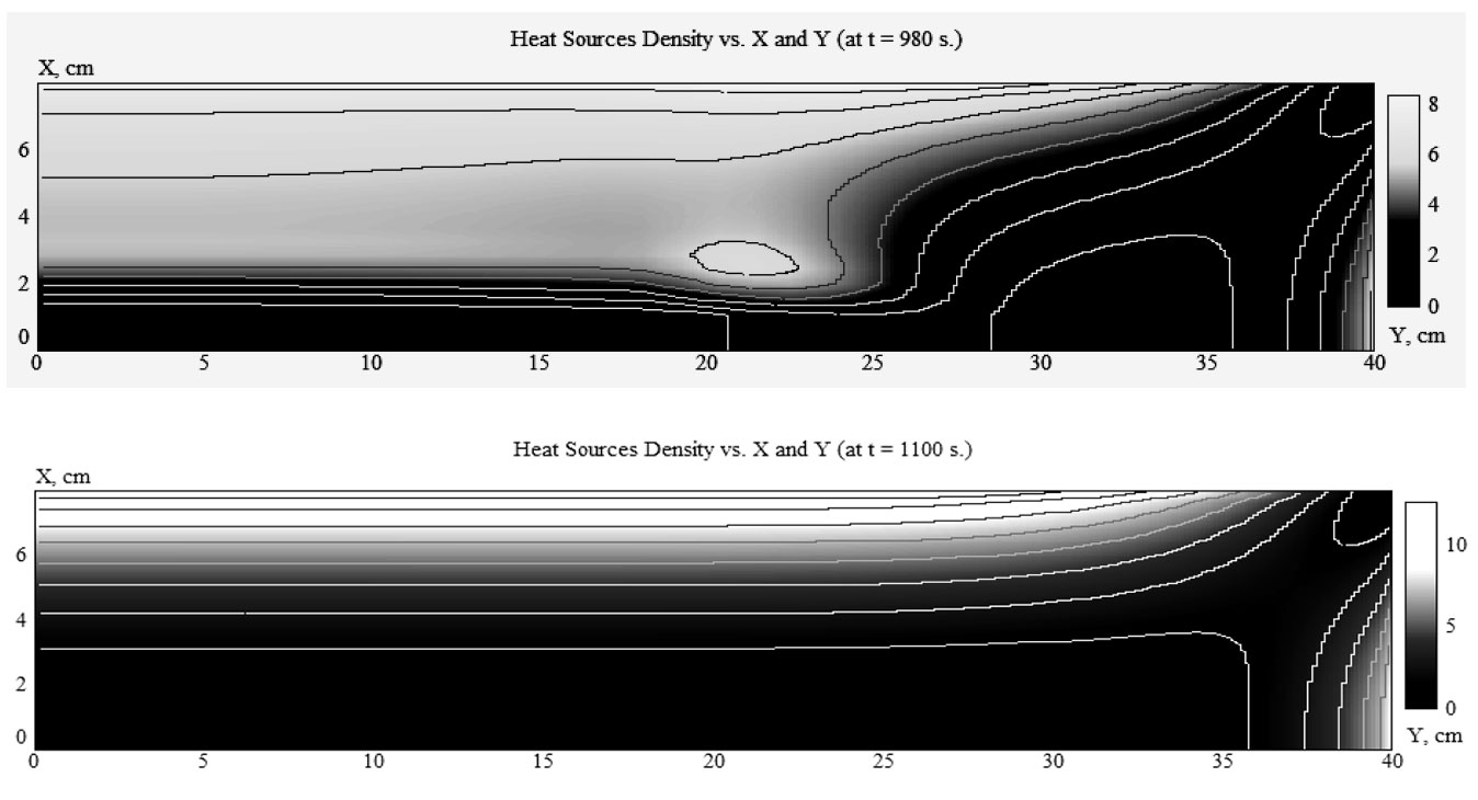
Volumetric power density distribution during the transient period is very odd, especially for a period 800-1000 sec (Fig. 3. Top). It is important to know a width of the edge-effect zone. In magnetic state it is about 2 cm, in hot state –around 10 cm, i.e. it equals to 0.625d or approximately 1.5δ. However at t= 980 sec this zone is around 16 cm.
Good understanding of edge effects is important for design of the slab heating process simplifying complete simulation of the heating process and the inductor design with account for thermal losses.
2.2 Example of optimal design of multi-stage process of large slab heating
Slab: Dimensions 20×120×200 cm, material –low carbon steel 1020. Required final temperature 1200 ± 50°C. Production rate is 33 t/hr.
Processing: A four-stage “isothermal” process was selected after multiple iterations. Stage one – accelerated heating at frequency 50 Hz; stage two – heating at 50 Hz to bring the surface temperature close to maximum level; stage three – final heating at 150 Hz for temperature distribution improvement in thickness and width of slab; stage four – holding slab in thermal chamber for final temperature conditioning. Heating time in each inductor 400 sec, holding time 200 sec, transportation time 10 sec. Inductor designs were different for good efficiency and matching to the source (line or inverter).
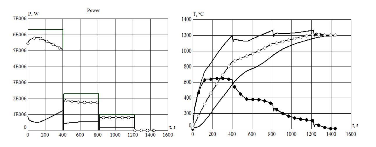
Powers at different stages and overall temperature dynamics for the central zone of slab are presented on Fig. 4.
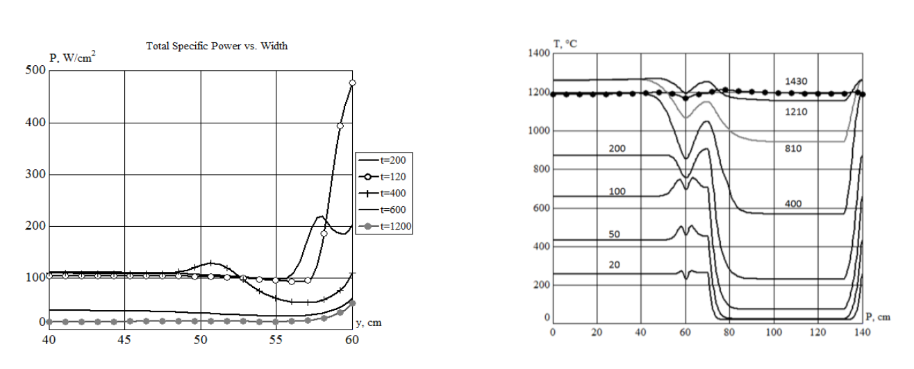
Fig. 5 shows distribution of absolute values of the total specific power in the width of slab and temperature distribution along the perimeter. Initial overheating of edge was compensated by lower p' at the end of the stage 1. Ratio d/δ for hot conditions is 2.8, i.e. slightly lower than optimal value for uniform adiabatic heating.
For this reason and for compensation of additional thermal losses from the slab side, frequency 150 Hz was selected for the final heating stage. Resulting temperature at the end of stage 3 corresponded to specifications. Stage 4 is an additional measure for very uniform temperature field (t = 1430 sec) and for compensation of short irregularities in the rolling mill demand for hot slabs.
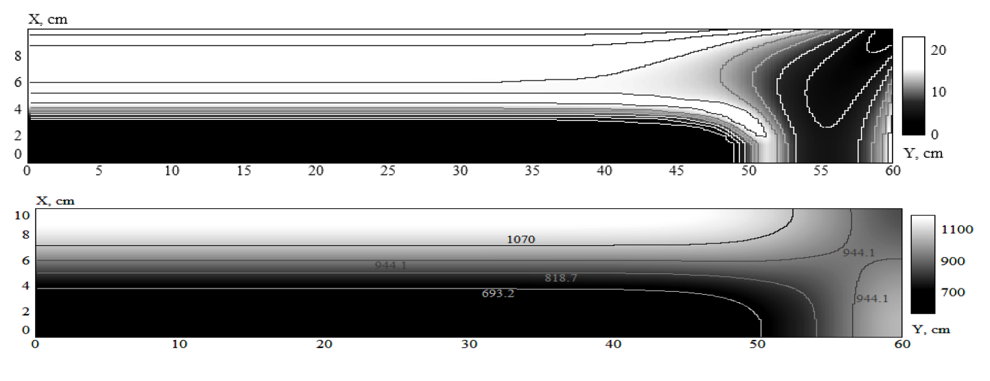
Fig. 6 gives additional information about power density and temperature distributions at the end of stage 1. Complete results of simulation include all the parameters of induction coils (currents, voltages, powers, capacitor batteries, etc.) and even requirements to the coil windings cooling systems. Calculated energy is rather small, less than 290 kWh/t.
Conclusion
- This study confirmed existing and provided new information about edge effects in heating slabs in longitudinal magnetic field.
- It was shown that the transient edge effect can lead to big edge zone underheating when heating magnetic slabs.
- Power variation due to edge effects can happen in the zone wider than the slab thickness.
- Obtained information may be used for optimal design of induction slab heaters.
References
[1] A. Muehlbauer: History of Induction Heating and Melting, Vulkan Verlag, 2008, p. 202.
[2] V. Peysakhovich: Calculation of impedances of inductively heated bodies with square and rectangular cross-section. Proceedings of VNIITVCh, Industrial applications of high frequency currents, Leningrad, Mashinostroyeniye, 1961, pp. 5-18 (in Russian).
[3] Zimin, L.S.: Particularities of induction heating for workpieces of rectangular form. Using of radio frequency current in electroheat. Leningrad, Mashinostroyeniye, 1973. pp. 25-34. (in Russian).
[4] V.S. Nemkov, V.B. Demidovich.: Theory and Calculation of Induction Heating Devices. Leningrad, Energoatomizdat, 1988, p. 280. (in Russian).
[5] Ivanov, A.N., Bukanin, V.A., Zenkov, A.E.: Advancements in program ELTA for calculation of induction heating systems. Proceeding of the International Conference on Heating by Electromagnetic Sources. Padua, May 21-24, 2013. pp. 345–351.
[6] Nemkov, V., Bukanin, V., Zenkov, A.: Learning and teaching induction heating using the program ELTA. Proceeding of the International Symposium on Heating by Electromagnetic Sources. Padua, May 18-21, 2010. pp. 99–106.
If you have more questions, require service or just need general information, we are here to help.
Our knowledgeable Customer Service team is available during business hours to answer your questions in regard to Fluxtrol product, pricing, ordering and other information. If you have technical questions about induction heating, material properties, our engineering and educational services, please contact our experts by phone, e-mail or mail.
Fluxtrol Inc.
1388 Atlantic Boulevard,
Auburn Hills, MI 48326
Telephone: +1-800-224-5522
Outside USA: 1-248-393-2000
FAX: +1-248-393-0277