Information
Authors: Robert Goldstein, Ethan Buchner, Robert Cryderman
Location/Venue: Colorado School of Mines
Download Full Presentation
Abstract
Dilatometry test systems are commonly used for characterizing the transformation behavior in steels and induction heating is commonly the heating source. In these systems, the steel test article is assumed to have a uniform temperature throughout the sample. This is a good assumption for slow heating rates with small samples, however, for induction hardening cycles this may or may not be accurate. Using computer models, it is possible to predict the temperature dynamics of the sample, both radially and axially, during the thermal processing cycle (heating and cooling).
O1 tool steel was utilized to characterize and model heating and cooling temperature gradients. Specimens instrumented with multiple thermocouples were induction heated and gas quenched. The test data and geometry were evaluated with 1-D and 2-D models to characterize transient temperature gradients. The goal of the modeling is to better characterize temperature corrections required when rapid heating and cooling processes are used to determine transformation behavior in induction hardenable steels.
Introduction
Most of the data on phase transformations for various steels available in the literature is for equilibrium conditions (tens or hundreds of thousands of seconds). In induction heat treating or other high power density heating methods (flame, laser, etc.), heating times are typically from 0.1 s to a few hundred seconds. The corresponding heating rates are about 5 °C/s to around 10,000 °C/s. Under these rapid heating conditions, the steel does not reach equilibrium conditions and therefore many of the corresponding curves from literature are not accurate. Both Ac1 and Ac3 for steels are sensitive to both heating rate and prior microstructure, but there is very little quantitative data available on these relationships [1].
Improved mechanical properties of steel components have been achieved using short austenitization cycles in combination with high cooling rates. Some of these improved results have been attributed to the ability to make composite bainite-martensite microstructures, but other results are for nearly 100% martensitic structures [2-4]. Depending upon the trials, different mechanisms have been proposed to explain the improved properties such as finer austenite grain size or better residual stress distributions [4]. However, more work needs to be done to better understand and quantify the conditions under which improved properties can be achieved in order to maximize the potential of induction heat treating.
Material Characterization Tools
The testing devices being used to study non-equilibrium transformation dynamics and subsequent properties at Colorado School of Mines include a Gleeble® 3500 resistance heating system with incorporated gas and/or liquid quench and a TA Instruments DIL805 dilatometer. The DIL805 uses a 3 kW, 150 – 400 kHz induction heating power supply for a heat source followed by gas quenching. Both of these devices have the capability to physically simulate induction heat treating processes on small sample sizes to characterize material behavior and subsequent properties. For both systems, temperatures are monitored during the process using thermocouples attached to the specimen surface. For the current study, only the DIL805 system is considered.
One case of heating and cooling was studied using the DIL805 dilatometer as follows:
- Heating rate of 50 °C/s
- Target temperature of 850 °C
- Holding time of 10 s
- Quenching media - helium
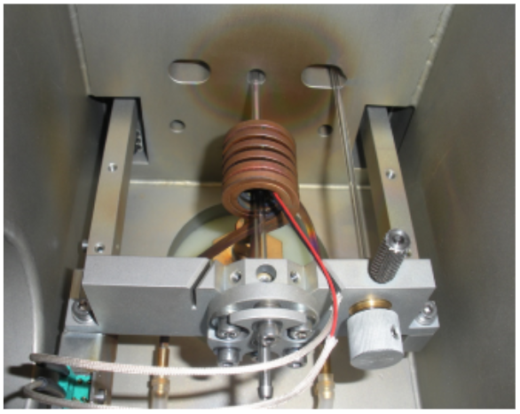
The goal of the computer models is to accurately predict the distributions of temperature in the sample during heating, holding, and cooling. The samples used in the test cell were 4 mm diameter by 10 mm long. The samples were held in place using quartz tubes. A picture of the test cell is shown in Fig. 1. The specimen is suspended between spring loaded hollow fused silica rods and a linear voltage displacement transducer is utilized to measure axial length changes. The unit is programmable such that linear heating and cooling rates can be attained within the limits of the power supply and quench capabilities. For this study, heating and holding were programmed followed by free quenching with helium.
In combination with the material tests, Fluxtrol, Inc. modeled the heating and cooling processes using ELTA [5] and Flux [6] software to understand the temperature distributions in the components. The reason for the modeling is to determine both the real temperature distributions and the “average” temperatures in the samples versus time, which can then be used to reinterpret and adjust the material behavior dynamics from the dilation measurements.
Model Development Strategy
1-D electromagnetic and thermal models were the first step in the evaluation process to understand the radial gradients of temperature in the part. The starting point for steel material properties important for simulation is the 0.45% C Steel hardened from the ELTA database [5].
The heating models were developed by adjusting the current supplied to the inductor so that the heating rate matched the desired value based upon the temperature at the surface of the center of the sample, the same point at which the dilatometer controls temperature. Power was then adjusted in the model to hold a constant surface temperature for the prescribed time.
The cooling models were developed by first simulating the heating cycle, but then adding on a cooling cycle to the end of the holding period. The gas cooling process was described by applying a convective heat transfer coefficient to the surface. The cooling models were run separately from the heating models, as there is currently not a standard option to have a different curve for specific heat capacity versus temperature for heating and cooling. Having different curves for specific heat capacity for heating and cooling is essential, as the steel goes through different phase transformations at different temperatures on heating and cooling and this affects the temperature dynamics.
After the initial cycle was developed, the measured surface temperatures were compared with the computer modelling results. The material properties were adjusted so that results correlated with the experimental data on temperature and power supply information. After fine tuning for the initial case, the results can be compared with other cases to ensure scalability of the models.
Once the material properties were determined using ELTA along with an approximate value for current versus time, 2-D models were run using Flux. Using Flux it is possible to analyze the axial temperature distribution. Depending upon the agreement, then either the material properties or the heat transfer coefficient can be adjusted to improve the data correlation. After achieving good correlation for a given trial, the models can be compared to other test conditions to validate the physical properties.
Results
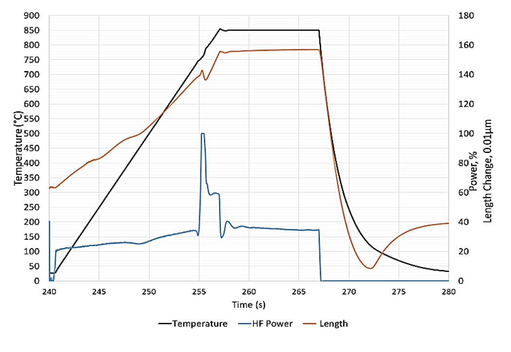
The baseline case selected for modelling was 50 °C/s heating rate, 850 °C austenitizing temperature, 10 s hold time and pressurized helium quench. A data plot showing temperature, “HF Power %,” and length versus time is shown in Fig. 2. Under the linear programmed heating conditions, the temperature of the sample tracked closely to the target temperature during the heating and isothermal holding process as shown in Fig. 2. When the steel reached approximately 750 °C, the generator “HF Power” increased to the maximum value of 100% as the steel temperature fell slightly below the programmed trendline. The sudden drop in the slope of the length vs time curve during heating indicates the start of the transformation from tempered martensite to austenite, and the return to the positive slope represents the completion of the transformation. After the steel was fully transformed to non-magnetic austenite, the power supply was able to once again provide the targeted heating rate, but at an increased power output compared to the level required for tempered martensite. The power level dropped again during the 10 s hold when the specimen reached the target austenitizing temperature. For this test, the generator ran at a high percentage of power during transformation and also for austenite heating, thus indicating that there is limited capability to deliver significantly higher heating rates above 750 °C for this configuration of coil and sample.
The cooling rate for the sample was much more rapid than the heating rate. The power was turned off with initiation of the helium quench. The deviation from the trend that occurred around 200 oC is due to the beginning of the martensitic phase transformation in the sample.
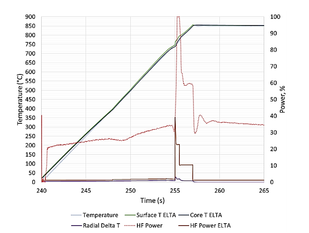
The results of the ELTA simulation are compared to the measured results for the heating process in Fig. 3. The results show that at the 50 °C/s heating rate, there is a relatively small difference between surface and core temperatures for this sample size. The maximum radial gradient during heating is around 20 °C and it occurs for only a short period of time around the phase transformation. During the holding process, the gradient is nearly zero.
Also, the shape of the “HF Power” curves agree well for the two cases. The agreement means that the enthalpy of phase transformation is likely close to correct for the O1 tool steel compared to the assumption of the value for 1045 in the ELTA database and no adjustment to the material properties are required.
In the ELTA modeling for this paper, only the power in the coil head is considered and the losses in the coil leads, heat station components, cable and generator are not included at this time. Even considering these factors, there remains a large difference between the predicted levels of power and the “HF Power” reported by the generator. This discrepancy can be caused by one of two factors:
- “HF Power %” is actually not percent power, but a percentage of another electrical parameter such as generator current
- Only a small fraction of the electrical power is delivered to the induction coil itself
Additional analysis is required to determine the source of the discrepancy, which may be done at a future date.
The cooling simulation results from ELTA are shown in Fig. 4. The heat transfer coefficient that was found to agree well with the measured data was 2200 W/m2K. While somewhat higher than published data for high pressure helium quenching (1000 – 1500 W/m2K is the typical range) [7], this can be explained by the small diameter of the rod, small diameter of the holes in the cooling tube in close proximity to the part (high gas velocity) and high pressure of the gas cylinder. All of these factors have the effect of increasing the heat transfer coefficient.
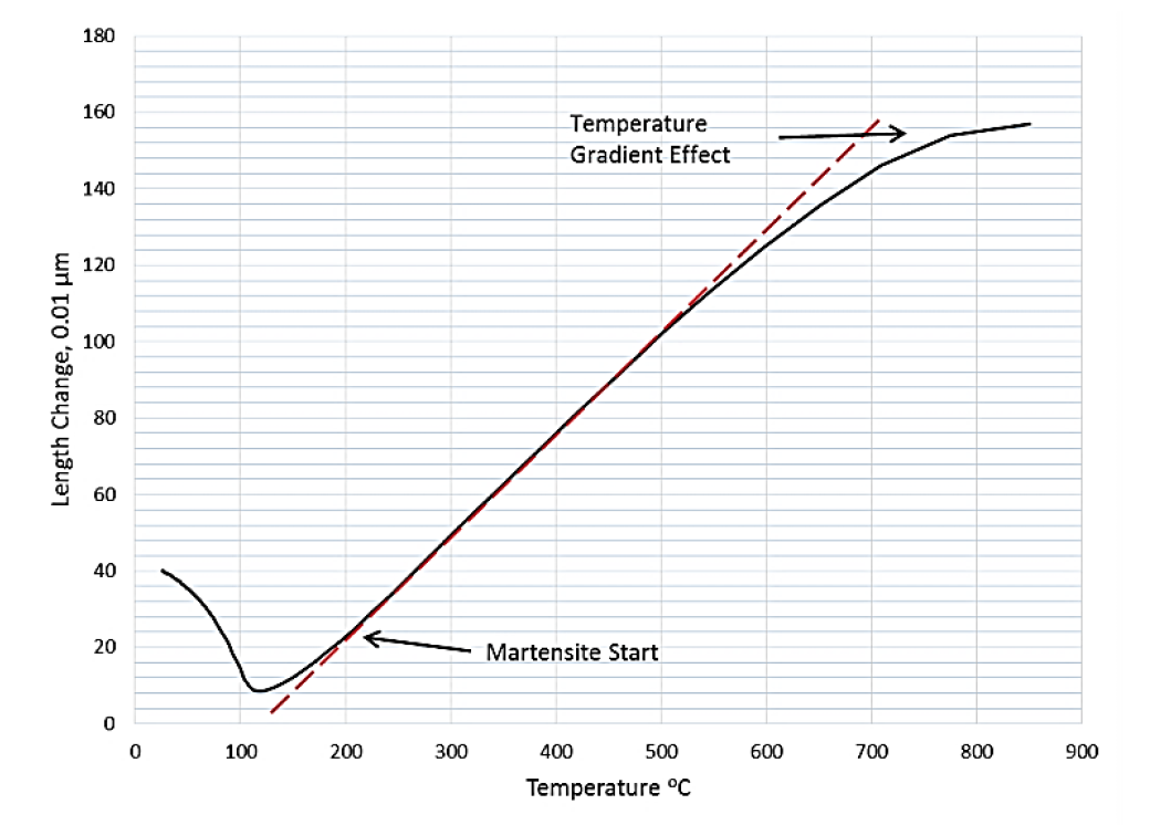
The specific heat capacity was adjusted in the temperature range of 150 °C and 50 °C so that the shape of the lower temperature cooling curve matched the experimentally measured values. This change was made to account for the transformation from austenite to martensite. The relationship between specimen length and temperature during helium quenching is shown in Fig. 5. The slope of the curve deviated from linear at just above 200 °C and became negative at 120 °C indicating the transformation to martensite. At low temperatures, there was some divergence between the calculated and actual temperature curves. This is because in ELTA, the default temperature for forced convection is 0 °C, whereas the real gas temperature was closer to 25 °C. It should be noted that the transformation to martensite was not complete at 25 °C, so the heat capacity adjustment may be appropriate only for this material.

The radial gradients are much higher for the cooling simulation than for the heating simulation. The maximum radial gradient is approximately 70 °C and occurs during the initial portion of the cooling process. This could be expected, because the rate of heat extraction is much faster than the heating rate and the cooling is purely a surface phenomenon, whereas power deposition during heating occurs at a certain depth into the sample. The effects of temperature gradients from surface to center and end to center can be seen in Fig. 5 where the measured specimen contraction did not begin to occur until after the initiation of the quench as measured by the surface thermocouple.
After studying the radial gradients in the samples and establishing material properties and cooling rates, the next step is to analyze the axial variations in the steel. Fig. 6 compares the temperature of the ends of the sample versus the center of the sample. The axial gradients within the sample on heating were much larger than the radial gradients during the heating process (approximately 2 times larger), with the ends being cooler than the center of the part. The gradients prior to the phase transformation grew approximately linearly while heating up to 750 °C, declined sharply, then grew again and stabilized at a lower differential throughout the high temperature heating and holding phase. This behavior can be explained by a combination of electromagnetic end effects and thermal losses (both radiative losses from the end and thermal conduction to the silica tube holding the part). Electromagnetic end effects should be slightly negative when the steel is magnetic at the beginning of the process and slightly positive when the steel is non-magnetic. It is important to note that during the heating and holding process, the temperature levels on the two ends of the sample were nearly identical. This means that the coil provided uniform power input and the thermal losses through the silica rods were consistent during the process.
For modeling in Flux, the system was assumed to be axisymmetric and half of the system was modeled axially as the part was centered in the coil. The geometry used for modeling is shown in Fig. 7.

The results of the Flux simulation are compared to the measured results for the heating process in Fig. 8. The results agree very well with the experimental measurements. The models show that there should be an axial gradient that grows up to the phase transformation, declines, then increases again and maintains a constant level through the holding phase. The level of declination at the phase transformation in the Flux model is less than the real experiments. This is likely due to the power supply hitting the HF power limit and not allowing the sample to continue heating at the desired target rate. Further refinement to the power input recipe in Flux would likely lead to a similar dynamic.
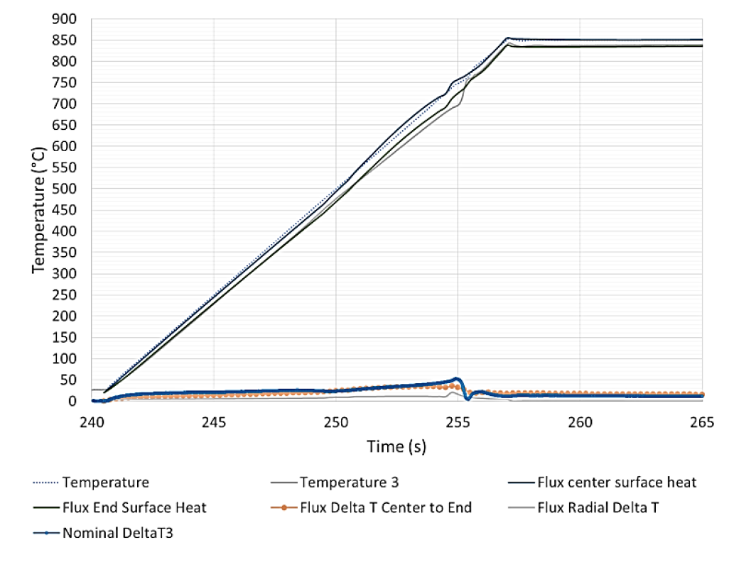
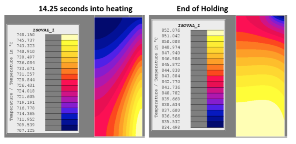
Fig. 9 shows a color shade representation of the temperature distribution in the sample at 14.25 seconds (maximum gradient near the phase transformation) and at the end of the 10 s holding process. During initial heating, the maximum temperature is on the surface in the center of the part. The temperature is lower near the ends of the part. The temperatures at the core of the sample are lower than on the surface. By the end of the holding phase, the core temperatures are actually slightly higher than the surface temperatures due to the balance between volumetric heat sources and thermal losses from the surface of the sample. However, the gradients are generally small and are concentrated in the area where the sample touches the silica rod.
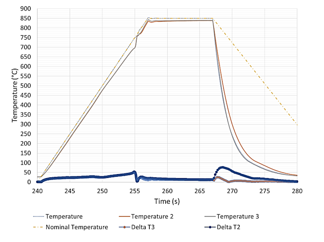
During the cooling process, the axial gradients were quite different from one end to the other (Fig. 6). These gradients were not present during the heating process, which means that their origin was from the cooling process. In Fig. 6, the absolute value of the temperature gradient is used. Fig. 10 gives a closer examination of the nominal temperature gradients end to end during cooling. On one end of the sample (Nominal Delta T3), the axial gradient inverted at the beginning of cooling (267 s) and climbed to a maximum level of approximately 25 °C. Shortly afterward, the temperature gradient inverted again and the ends were then cooler than the center of the part, before the gradient trended to zero. For the other end of the part (Nominal Delta T2), after the initial inversion the gradient between the center and part continued to grow to around 75 °C and then trended to zero during the cooling process. The likely explanation for this is that there was a significant gradient in the heat transfer coefficient in the length of the sample. This is further demonstrated when graphing the nominal temperature difference between the two ends of the sample (Nominal DeltaT2 to T3). There were only minor, intermittent gradients during the heating process, but very large gradients during the cooling process.
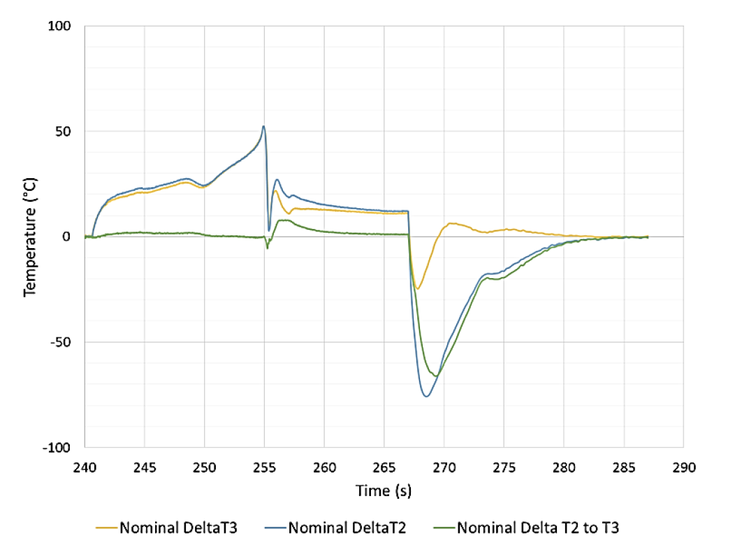
Fig. 11 shows the calculated and actual cooling curves. For the cooling simulation, a constant heat transfer coefficient in length was used and extended along the length of the surface of the silica rod. Temperature 2 was not included in this comparison. The shape of the cool down curves in the center of the part matches well, implying good agreement on the level of heat transfer coefficient and the martensitic phase transformation impact. Also, with a gas temperature of 25 °C, the final cooling agreement is excellent between the models and experiments in the center of the part.
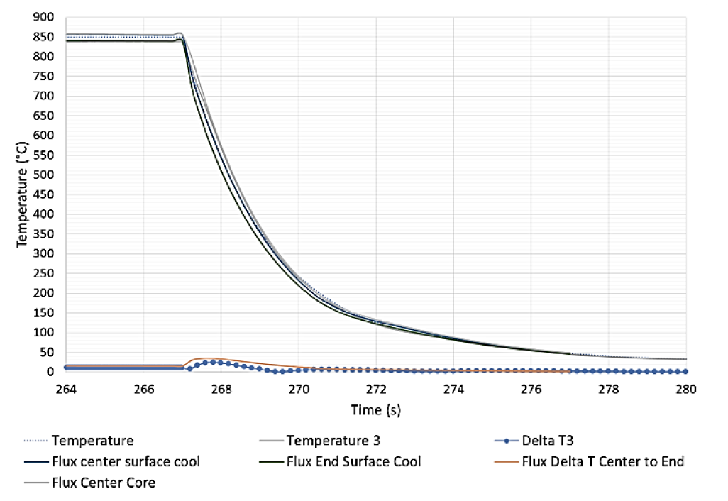
On the ends of the part, there is some disagreement in the cooling predictions. Fig. 12 shows the nominal temperature gradients from end to center of the part during the cooling process from simulation and experiments. The models (with a uniform heat transfer coefficient in length) predict that the center surface should be higher throughout the process, rather than undergoing the inversion during the initial portion of the cooling. The reason for the initial rise in gradient can be explained by the fact that there are two additional cooling mechanisms present on the ends of the sample compared to the middle:
- radiant loss from the end surface of the sample
- conductive cooling from the silica rods.
After the very rapid initial cooling, the curves agree very well during the final portions of the cooling process.
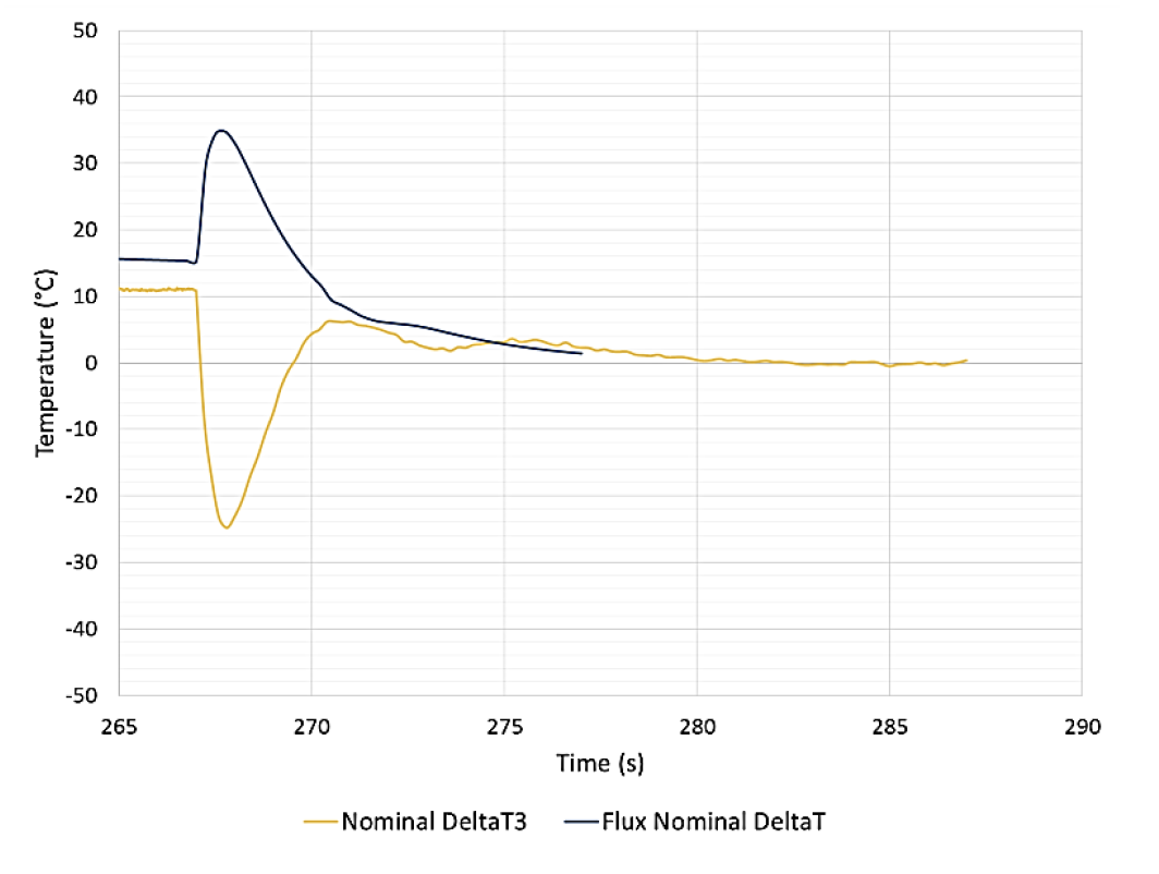
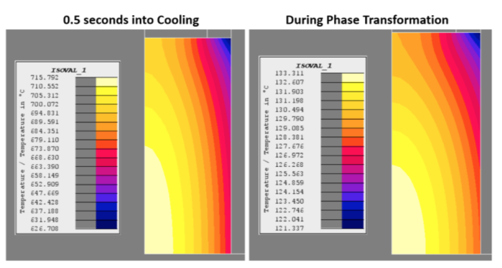
Fig. 13 shows a comparison of the color shade of the temperature distribution 0.5 seconds into the cooling process along with one where the surface temperature is 130 °C (during the phase transformation). During the initial phases of cooling, there are both significant axial and radial gradients in the component (span of temperature approximately 90 °C, with most of the mass substantially warmer than the central surface). During these portions of the cooling process, it is necessary to recalculate the equivalent temperatures in order to adjust the dilatometer results to compensate for the thermal lag effect shown in Fig. 5 and described in the literature [8]. However, during the phase transformation with transformation heat evolution, thermal gradients should be smaller for a sample exposed to uniform surface cooling conditions.
Summary
A modeling study was conducted to characterize the full temperature distributions occurring during testing being conducted using a TA Instruments DIL805 dilatometer under 50 °C/s heating and helium cooling conditions for O1 tool steel. Models were developed that accurately predict heating dynamics and the results match very well to measured values of temperature.
Cooling simulations showed excellent agreement for the temperature dynamics on the center surface of the part. They also showed that the gradients present during the initial phases of cooling were much larger than for the heating process due to the more rapid rate of surface temperature change. This phenomenon was observed experimentally in the dimensional movement measurements with helium cooling.
Temperature measurement on the ends showed a significant axial temperature gradient in the part during cooling. During the initial phases of cooling, the temperature on both ends of the sample were higher than the temperature in the center of the component. During later stages of cooling, the temperature on one end of the component stayed warmer than the center while the other end of the component became cooler than the center. Both temperatures converged on the same final temperature. Models using a uniform convective heat transfer coefficient, showed that the center temperature should always exceed the temperature of the ends of the samples during cooling. More study is required to better understand the source of the unexpected component cooling behavior. Significant end to end gradients were not present during the heating process. The current hypothesis for this is a gradient in the heat transfer coefficient along the surface of the component is the source of the gradients during cooling. More study is required to better quantify this behavior so that it may be either resolved through improved cooling system design or to incorporate the non-uniformity into the models.
It is important to remember that 50 °C/s is a relatively slow heating rate and helium quenching is not as rapid as water/polymer spray quenchants typically used in industrial induction hardening applications. If the heating and/or cooling rate(s) are increased, the gradients present will likely expand proportional to the rate of temperature change. Even with the relatively slow heating and cooling rates, the results show that there are significant temperature gradients that occur during transient periods of the cycle that need to be accounted for when analyzing dimensional movement measurements. Results should be adjusted using an “average” temperature value for the volume calculated from the modeling results.
The results also show, that the unit will have difficulty in achieving significantly higher heating rates common during induction hardening processes during and above the phase transformation due to the unit reaching an “HF Power” limit. There is a significant difference in the modeled power levels and the available power from the induction heating power supply. More study needs to be done to understand the difference in order to see if there is a way to provide increased heating rates through and above the phase transformation to better simulate steel behavior under induction heating conditions.
Future studies will involve extending this study to other sample sizes, materials and rates of temperature change to better characterize steel behavior under induction hardening conditions. Finally, the authors are currently working with the Altair development team to develop a method to take into account the variations in specific heat capacity versus temperature that occur during induction hardening applications so that one model may be used for both heating and cooling analysis using Flux.
Acknowledgement
The authors acknowledge the support of Fluxtrol, Inc. and the corporate sponsors of the Advanced Steel Processing and Products Research Center, an industry/university cooperative research center at the Colorado School of Mines.
References
[1] Clarke, K. D., and Van Tyne, C. J., The Effect of Heating Rate and Prior Microstructure on Austenitization Kinetics of 5150 Hot-Rolled and Quenched and Tempered Steel, Proceedings of MS&T 2007, September, 2007.
[2] Vigilante, G., Hespos, M. and Bartolucci, S. “Evaluation of Flash Bainite in 4130 Steel,” Technical Report ARWSB-TR-11011, July 2011, Armament Research, Development and Engineering Center, Weapons and Software Engineering Center Benet Laboratories.
[3] Cryderman, R. L. and Speer, J. “Microstructure and Notched Fracture Resistance of 0.56% C Steels After Simulated Induction Hardening,” Proc., 29th ASM Heat Treating Society Conference, Oct 24-26, 2017, Columbus, Ohio.
[4] Fukuzawa, K.,Misaka, Y., and Kawasaki, K.,, “The Effects of Grain Refinement on the Fatigue Properties of Induction Hardened Cr-Mo Steel,” Proc., 17th IFHTSE Congress, Oct 27-30, 2008, Kobe, Japan.
[5] New Solutions Group, “Software for Induction Heating,”www.nsgsoft.com
[6] Altair, “Hyperworks,” www.altairhyperworks.com
[7] Lin, M., “Gas Quenching With Air Products’ Rapid Gas Quenching Gas Mixture,” Air Products, http://www.airproducts.com/~/media/Files/PDF/industries/metals/metals-gas-quenching-air-products-rapid-gas-quenching-gas-mixture.pdf
[8] Cryderman, R. L. and Ballard, T., “Short Time Austenitizing Effects on the Hardenability of Some 0.55 wt. pct. Carbon Steels,” Proc., 24th IFHTSE Congress, June 26-29, 2017, Nice, France.
If you have more questions, require service or just need general information, we are here to help.
Our knowledgeable Customer Service team is available during regular business hours to answer your questions in regards to Fluxtrol products, pricing, ordering, and other information. If you have technical questions about induction heating, material properties, or engineering and educational services, please contact our experts by phone, e-mail or mail.
Fluxtrol Inc.
1388 Atlantic Boulevard,
Auburn Hills, MI 48326
Telephone: +1-800-224-5522
Outside USA: 1-248-393-2000
FAX: +1-248-393-0277