Toll Free


Information
Authors: Tareq Eddir, Robert Goldstein, Ethan Buchner, Emmanuel De Moor, Robert Cryderman
Location/Venue: IFHTSE TPIM 18 Spartanburg, South Carolina
Download Full Paper
Download Presentation PDF
Abstract
Dilatometry test systems are commonly used for characterizing the transformation behavior in steels and induction heating is frequently selected as the heating source. In these systems, the steel test specimen is assumed to have a uniform temperature throughout the sample. This is a good assumption for slow heating rates with small specimens, however, for induction hardening heating rates this may not be accurate. Using computer models, it is possible to predict the temperature dynamics of the sample, both radially and axially, during heating.
O1 tool steel in the quenched condition was utilized to characterize and model heating temperature gradients. The case of a 50°C/s heating rate was presented previously [1]. In this study, specimens instrumented with multiple thermocouples were induction heated at rates up to 500 °C/s. The test data and geometry were evaluated with 2-D models to characterize transient temperature gradients. The goal of the modeling is to better characterize temperature corrections required when rapid heating is used to determine transformation behavior during rapid induction heating. This paper presents the data for faster heating rates and quantifies the impact of the different heating rates on the dynamic temperature distributions in the sample.
Introduction
Most of the data on phase transformations for various steels available in the literature is for equilibrium conditions corresponding to prolonged holding times on the order of many hours. In induction heat treating or other high power density heating methods (flame, laser, etc.), heating times are typically from 0.1 s to a few hundred seconds. The corresponding heating rates are about 5 °C/s to around 10,000 °C/s. Under these rapid heating conditions, the steel does not reach equilibrium conditions and therefore many of the corresponding curves from literature are not accurate. Both Ac1 and Ac3 for steels are sensitive to both heating rate and prior microstructure, but there is very little quantitative data available on these relationships [2].
Improved mechanical properties of steel components have been achieved using short austenitization cycles in combination with high cooling rates. Some of these improved results have been attributed to finer austenite grain sizes with nearly 100% martensitic structures [3-4]. Depending upon the trials, different mechanisms have been proposed to explain the improved properties such as finer austenite grain size or better residual stress distributions [4]. However, more work needs to be done to better understand and quantify the conditions under which improved properties can be achieved in order to maximize the potential of induction heat treating.
Material Characterization Tools
The testing devices being used to study non-equilibrium transformation dynamics and subsequent properties at Colorado School of Mines include a Gleeble® 3500 resistance heating system with incorporated gas and/or liquid quench and a TA Instruments DIL805 dilatometer. The DIL805 uses a 3 kW, 150 – 400 kHz induction heating power supply for a heat source followed by gas quenching. Both of these devices have the capability to physically simulate induction heat treating processes on small sample sizes to characterize material behavior and subsequent properties. For both systems, temperatures are monitored during the process using thermocouples attached to the specimen surface. For the current study, only the DIL805 system is considered.
The cases of heating were studied using the DIL805 dilatometer as follows:
- Heating rates of 0.1, 0.5, 5, 50, and 500 °C/s
- Target temperature of 900 °C
- Holding time of 1 s
- Quench was not studied
The goal of the computer models is to accurately predict the distributions of temperature in the sample during heating and holding. The specimens used in the test cell were 4 mm diameter by 10 mm long. The samples were held in place using fused silica rods. A picture of the test cell is shown in Fig. 1. The specimen is suspended between spring loaded hollow fused silica rods and a linear voltage displacement transducer is utilized to measure axial length changes. The unit is programmable such that linear heating rates can be attained within the limits of the power supply. For this study, heating and holding were programmed. Three thermocouples were used to measure and control the temperature of the specimen during heating and holding. Considering the symmetry of the system, the thermocouples were placed at the center (TC1), quarter length (TC2), and end of the specimen (TC3), with TC1 used for temperature control. Figure 1: Dilatometer showing thermocouple leads, specimen suspended between fused silica rods, outer water cooled induction coil, and inner gas quenching coil.
In combination with the material tests, Fluxtrol, Inc. modeled the heating process using Flux 2D [5] software to understand the temperature distributions in the components. The reason for the modeling is to determine the real temperature distributions in the samples versus time, which can then be used to reinterpret and adjust the material behavior dynamics from the dilation measurements.
Model Development Strategy
2-D electromagnetic and thermal models were used to understand the temperature gradients in the specimen. The material properties important for simulation were developed in a previous study [1].
The heating models were developed by adjusting the current supplied to the inductor so that the heating rate matched the desired value based upon the temperature at the surface of the center of the sample, the same point at which the dilatometer controls temperature. The material properties and heat transfer coefficient were modified until the experimental and model results agreed [1]. After the material properties were determined, the model’s agreement with the experimental results was evaluated by comparing temperature results from the two other thermocouples.
Results
The cases selected were for 0.1, 0.5, 5, 50, and 500 °C/s heating rate, 900 °C austenitizing temperature, and 1 s hold. A data plot showing temperature data for TC1, TC2, and TC3 for the 0.1 °C/s is shown in Fig. 2. The plot has six graphs, experimental and model results for each of the thermocouples. Due to the very slow heating rate, the temperature gradients are small, with no significant axial temperature gradients observed. The results also show close agreement between the experimental and model results. Figure 2: Dilatometer and model data for 0.1 °C/s heating rate, target temperature of 900 °C, 1 s hold.
After the model’s external temperatures for the specimen were compared, the data for gradients in the specimens were extracted from the models, volumetric average temperatures were also calculated. A plot for the temperature gradient and temperature difference was plotted vs time is shown in Fig. 3 for the 0.1 °C/s case. The value for the gradient is calculated by subtracting the specimen’s minimum temperature from the maximum temperature at any point. The value for the difference is calculated by subtracting the average temperature from the control temperature, TC1, at any point. Figure 3: Temperature gradients and differences in the specimen from the model for the 0.1 °C/s case.
The results in Fig. 3 show the maximum temperature gradient is 8.1 °C and a final gradient temperature of 7.2 °C. The temperature difference data show a maximum of 3.2 °C and a final difference of 1.0 °C between the TC1 and the average temperature. The maximum gradient and difference occur leading up to the Curie transformation. Temperature distribution map in the specimen at the end of the temperature hold for the 0.1 °C/s is shown in Fig. 4. Figure 4: Temperature distribution map at the end of the temperature hold for the 0.1°C/s case.
The temperature distribution map in Fig. 4 shows uniform temperature distribution with the max temperature at the core of the specimen, resulting from the radiative heat loss at the exterior of the specimen. Additionally, radiation and conduction through the silica rods result in the ends of the specimen having the lowest temperature.
A data plot showing temperature data for TC1, TC2, and TC3 for the 0.5 and 5 °C/s is shown in Fig. 5. Figure 5: Dilatometer and model data for 0.5 and 5 °C/s heating rate, target temperature of 900 °C, 1 s hold.
The results in Fig. 5 show the measured and modeled temperature graphs for each of the three thermocouples for both the 0.5 and 5 °C/s cases. The results show close agreements between the model and measured data. The data also show minimal temperature gradients between the three thermocouples for each case, indicating a small axial temperature gradient. A plot showing the temperature gradient and temperature difference for the 0.5 and 5 °C/s is shown in Fig 6. Figure 6: Temperature gradients and differences in the specimen from the model for the 0.5 and 5 °C/s cases.
The results in Fig 6 show a maximum and final temperature gradient of 7.9 °C for the 0.5 °C/s case. The 5 °C/s case has a maximum temperature gradient of 13.2 °C and a final temperature gradient of 12.3 °C/s. The results also show a maximum temperature difference of 2.9 °C and a final temperature difference of 1.3 °C for the 0.5 °C/s case, while the 5 °C/s case had a maximum and final temperature differences of 5.5 and 2.6 °C, respectively. Temperature distribution maps for the end of heat for both cases are shown in Fig 7. Figure 7: Temperature distribution map at the end of the temperature hold for the 0.5°C/s case on the left and the 5 °C/s case on the right.
The temperature distribution maps in Fig. 7 show uniform temperature distribution with the maximum temperature at the core of the specimen for both cases, as with the 0.1 °C/s case. The 0.5 °C/s case shows higher temperature uniformity than the 5 °C/s case. Both cases have a lower temperature at the end of the specimen, with more axial gradients for the 5 °C/s case.
A data plot showing temperature data for TC1, TC2, and TC3 for the 50 and 500 °C/s is shown in Fig. 8. Figure 8: Dilatometer and model data for 50 and 500 °C/s heating rate, target temperature of 900 °C, 1 s hold.
The results in Fig. 8 show the measured and modeled temperature graphs for each of the three thermocouples for both the 50 and 500 °C/s cases. For both cases the heating rate is lower leading up to the Curie point, while the 500 °C/s case continues to heat at a lower rate past the Curie point. The lower heating rates are believed to be a result of the machine reaching a current limit. As a result, the models were designed to follow the temperature curves from the experiments, rather than a programmed heating rate. The results show close agreements between the model and measured data. The data also show that the axial temperature gradients are minimal at the end of the temperature hold but they are significant during the heating stage, especially around the Curie point. They are also greater than what is observed for the lower heating rates. A plot showing the temperature gradient and temperature difference for the 50 and 500 °C/s is shown in Fig 9. Figure 9: Temperature gradients and differences in the specimen from the model for the 50 and 500 °C/s cases.
The results in Fig 9 show a maximum temperature gradient of 37.2 °C and a final temperature gradient of 22 °C for the 50 °C/s case. The 500 °C/s case has a maximum temperature gradient of 154.7 °C and a final temperature gradient of 25 °C. The results also show a maximum temperature difference of 18.8 °C and a final temperature difference of 5.0 °C for the 50 °C/s case, while the 500 °C/s case had a maximum and a final temperature differences of 82.2 °C and 6.7 °C, respectively. It is expected that if the heating rate could be maintained after Curie for the 500 °C/s case the gradients will be higher at the end of heating. Temperature distribution maps for the end of heating for both cases are shown in Fig 10.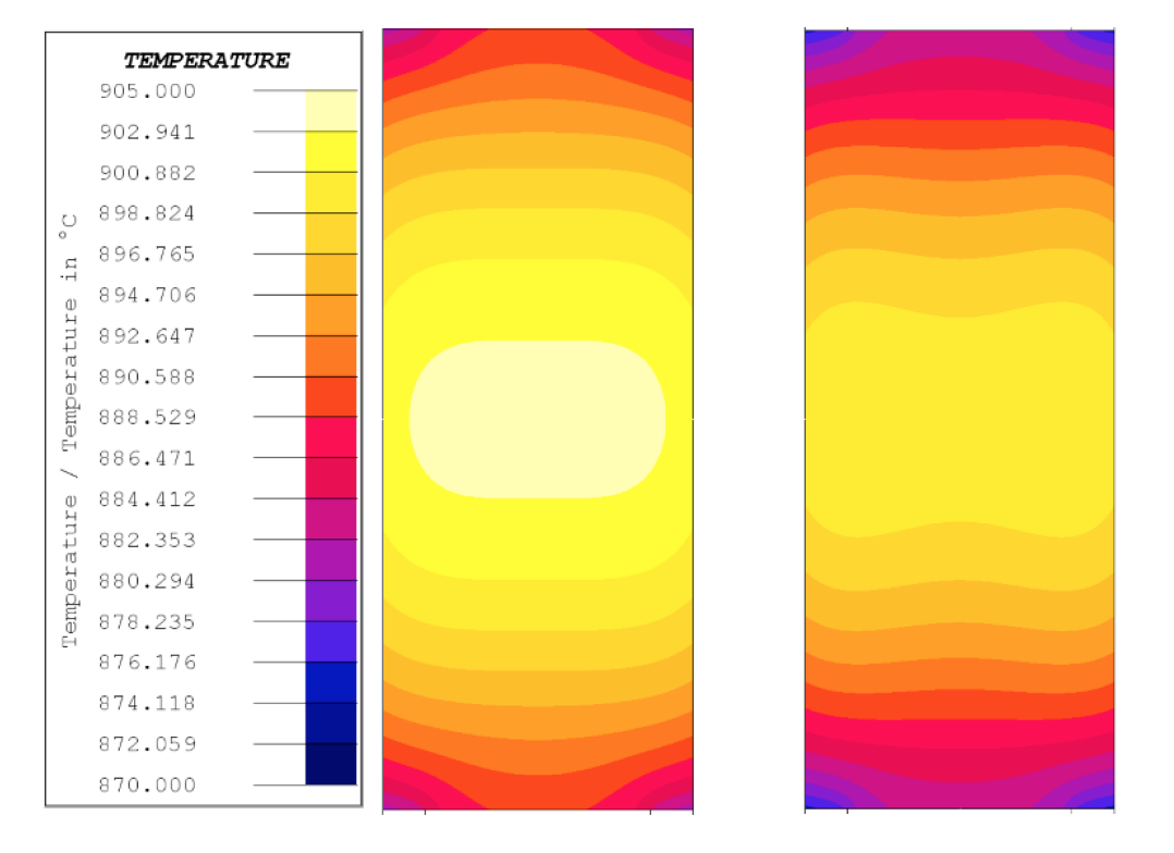 Figure 10: Temperature distribution maps at the end of the temperature hold for the 50°C/s case on the left and the 500 °C/s case on the right.
The temperature distribution maps in Fig. 10 show temperature distribution at the end of heat, with the maximum temperature at the core of the specimen for both cases, as with the other cases. Both cases have higher axial temperature gradients than the lower heating rate cases, with the 500 °C/s case having the highest gradients of all cases. A temperature distribution map for the 500 °C/s case when the TC1 is at 760°C is shown in Fig. 11. Figure 11: Temperature distribution map for the 500 °C/s case when TC1 is 760 °C.
The temperature distribution map in Fig. 11 shows the gradients in the specimen for the 500 °C/s case when they are the greatest. The results show a large axial calculated temperature gradient, with TC1, TC2, and TC3, measuring 760, 733, and 657 °C, respectively. The measured data for TC1, TC2, and TC3 are 760, 727, and 648 °C, respectively. The lowest calculated temperature at that time is 612 °C, at the center at the end of the specimen.
A plot showing the maximum temperature gradient, final temperature gradient, maximum temperature difference, and final temperature difference for all heating rates is shown in Fig 12. Figure 12: Maximum and final temperature gradients and differences plotted for every heating rate.
The results in Fig. 12 show the maximum temperature gradient increases with the heating rate. At the lower heating rates, the maximum temperature gradient and final temperature gradients are very close. For the higher heating rates, from 5 to 500 °C, the maximum gradient occurs around the Curie point, then the temperature gradients reduce. The plot also shows that the final temperature gradients increase with the heating rate, but they plateau to around 25 °C. The results show the final temperature gradients for the 50 and 500 °C/s are 22 and 25 °C, respectively.
The maximum temperature difference results in Fig. 12 show an increase with the heating rate, while the final temperature difference plateaus to around 7 °C. The minimum temperature difference results also indicate radial temperature uniformity, which is also observed in the temperature distribution maps.
A plot showing the average temperature vs the model’s TC1 temperature for every case is shown in Fig 13.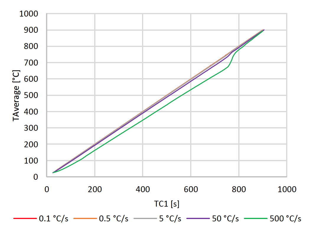 Figure 13: Temperature average vs TC1 temperature for every case.
The results in Fig. 13 show the average temperature for the specimen, as calculated from the model, plotted against TC1 from the model. The results show insignificant difference between the average temperature and TC1 for the lower heating rates. The results for the 50 °C/s case show the difference reaches the maximum around the Curie temperature, or the beginning of the transformation to non-magnetic austenite. After transformation, the difference between the average temperature and the control temperature reduces. The results for the 500 °C/s show great temperature gradients. The temperature difference is significant from the beginning of the heating process and reaches the maximum around the Curie point. After transformation, the temperature difference reduces.
During the heating process the specimen’s length was measured for each case. Dilatometry curves for different cases are shown in Fig 14. Figure 14: Dilatometry curves for the 0.1, 0.5, 5, and 5 °C/s heating rates.
The results in Fig. 14 show the dilatometry results for all the heating rates, except the 500 °C/s. Setup measurement issues resulted in noisy dilatometry data for the 500 °C/s heating rate, so the results were omitted. The dilatometry results for the 50 °/s heating rate were plotted against the measured TC1 and against the average temperature, as calculated from the model.
The lower heating rates show the deviations from linearity in the dilation slopes at the lower temperature values, approximately less than 500 °C, this is due to tempering, as the incoming samples have martensitic structures. The deviations in the dilatation slope for the 50 °C/s heating rate are less pronounced as the higher heating rate doesn’t allow for complete tempering.
The results also show a shift in Ac1 and Ac3 with heating rate. The results show Ac1 for the 0.1, 0.5, 5, and 50 °C/s is approximately 734, 734, 746, and 762 °C, respectively. While Ac3 is 760, 766, 779, and 800 °C. Correcting the 50 °C/s data for the average specimen sample instead of the control temperature yields Ac1 and Ac3 of 757 °C and 794 °C, respectively. The values for Ac1 and Ac3 are expected to continue to increase with higher heating rates with larger corrections required.
Measured and corrected Ac1 and Ac3 values are shown in Table 1. The results show the corrected values for the 0.1 and 0.5 °C/s cases are identical to the measured values. The corrected values for the 5 °C/s case show a shift of 3 °C and 1 °C for Ac1 and Ac3 from the measured values, respectively. The values for the 50 °C/s show an increase in the shift between the measured and corrected values.
Table 1. Measured and Corrected Transformation Temperatures °C
| Heating Rate, °C/s | Measured | Corrected | ||
|---|---|---|---|---|
| Ac1 | Ac3 | Ac1 | Ac3 | |
| 0.1 | 734 | 760 | 734 | 760 |
| 0.5 | 734 | 766 | 734 | 766 |
| 5 | 746 | 779 | 743 | 778 |
| 50 | 762 | 800 | 757 | 794 |
The results in Table 1 indicate that for the lower heating rates the measured temperature can be considered the same as the average specimen temperature. Additionally, the measured Ac1 and Ac3 values can be considered the same as the corrected values. The results also show that for the 50 °C/s case the values for Ac1 and Ac3 increase, so does the difference between their measured and corrected valued. This behavior is also expected for higher heating rates.
Results for the change in dilation with temperature plotted as the first derivative with respect to temperature is shown for the different cases in Fig 15. The shift in measured transformation start and finish temperatures is clearly evident. Figure 15: Change in dilation with respect to temperature for the 0.1, 0.5, 5, and 50 °C/s.
Summary
A modeling study was conducted to characterize temperature gradients in induction heated dilatometry O1 tool steel specimens using TA Instruments DIL805 at 0.1, 0.5, 5, 50, and 500 °C/s heating rates to 900 °C with a 1 s hold. Models were developed that accurately predict heating dynamics and match the measured values of temperature very well.
Temperature measurements and model results show insignificant axial and radial temperature gradients at the lower heating rates, but the gradients increase with higher heating rates. The results show the highest gradients occur around the Curie temperature. At 50 °C/s and 500 °C/s the maximum temperature gradients in the specimens were approximately 37 and 155 °C, respectively. At the end of the holding stage, the radial temperature gradients were very minimal, but higher axial temperature gradients up to 25 °C remained.
The modeling results show that the final temperature gradients initially increase with the heating rate, but eventually plateau. The final difference in gradients between the 50 °C/s and the 500 °C/s can be considered minimal. However, the gradients during the heating, especially leading up to the Curie point or Ac1, continued to increase with the heating rate, even at the higher heating rate.
It is important to note that for the 50 and 500 °C/s cases, the dilatometer did not maintain those heating rates for the entirety of the experiments, and it is expected that the gradients will be even greater if the rate is maintained.
The study shows the assumption of a uniform temperature distribution for induction heated specimens is not always appropriate. For the lower heating rates investigated, 0.1, 0.5, and 5 °C/s the gradients may be considered negligible enough to assume temperature uniformity. For the higher heating rates investigated, 50 and 500 °C/s, the gradients should not be considered negligible and temperature uniformity should not be assumed, especially around the Ac1 to Ac3 and Curie temperature.
The dilatometry results show a shift in Ac1 and Ac3 with heating rates. The shift is also expected to continue for heating rates higher than the 50 °C/s shown. By combining the modeling average temperature and the measured TC1, it was shown that while Ac1 and Ac3 are shifted to higher temperatures, the values corresponding to the measured temperature are greater than those corresponding to the average temperature. In other words, the surface mounted thermocouple over estimates the transformation temperature during heating due to the thermal lag in the majority of the specimen. This behavior is expected to be greater for higher heating rates.
The study shows that using equilibrium transformation data or data from slow heating rates does not apply for induction heating dilatometry experiments with high heating rates, especially at or above 50 °C/s.
Future studies will look at different sample geometries and frequencies to investigate the effects on the radial and axial temperature gradients and dilatometry data for heating rates above 50 °C/s. Future studies will also look at using dilatometry experiments to determine transformation data for modeling material characteristics at different heating rates.
Acknowledgement
The authors acknowledge the support of Fluxtrol, Inc. and the corporate sponsors of the Advanced Steel Processing and Products Research Center, an industry/university cooperative research center at the Colorado School of Mines.
References
[1] Buchner, E., Cryderman, R. L., and Goldstein R., “Modeling of Short Time Dilatometry Testing of High Carbon Steels,” Proc., 29th ASM Heat Treating Society Conference, Oct 24-26, 2017, Columbus, Ohio.
[2] Clarke, K. D., and Van Tyne, C. J., The Effect of Heating Rate and Prior Microstructure on Austenitization Kinetics of 5150 Hot-Rolled and Quenched and Tempered Steel, Proceedings of MS&T 2007, September, 2007.
[3] Cryderman, R. L. and Speer, J. “Microstructure and Notched Fracture Resistance of 0.56% C Steels After Simulated Induction Hardening,” Proc., 29th ASM Heat Treating Society Conference, Oct 24-26, 2017, Columbus, Ohio.
[4] Fukuzawa, K.,Misaka, Y., and Kawasaki, K., “The Effects of Grain Refinement on the Fatigue Properties of Induction Hardened Cr-Mo Steel,” Proc., 17th IFHTSE Congress, Oct 27-30, 2008, Kobe, Japan.
[5] Altair, “Hyperworks,” www.altairhyperworks.com
If you have more questions, require service or just need general information, we are here to help.
Our knowledgeable Customer Service team is available during business hours to answer your questions in regard to Fluxtrol product, pricing, ordering and other information. If you have technical questions about induction heating, material properties, our engineering and educational services, please contact our experts by phone, e-mail or mail.
Fluxtrol Inc.
1388 Atlantic Boulevard,
Auburn Hills, MI 48326
Telephone: +1-800-224-5522
Outside USA: 1-248-393-2000
FAX: +1-248-393-0277