Information

Authors: Andrew L. Banka (Airflow Sciences Corporation), Robert C. Goldstein (Fluxtrol Inc.), Robert L. Cryderman (Colorado School of Mines), Tareq Eddir (Fluxtrol Inc.), Andrew Senita (Airflow Sciences Corporation)
Location/Venue: ASM HTS Heat Treat 2019 Detroit, Michigan

Download Full Paper
Download Presentation PDF

Abstract

Dilatometry test systems are commonly used for characterizing the transformation behavior in steels using induction heating for the heating source and gas flow for the cooling source. In these systems, the steel test article is assumed to have a uniform temperature throughout the sample. The accuracy of this assumption depends on the design of the induction heating and gas cooling systems, as well as the time scales for heating and cooling. Previous papers by the authors have shown the variations in temperature that occur during heating and cooling for a TA Instruments DIL805 dilatometer (dilatometer).

Investigations were carried out for development of an improved heating/cooling system for this dilatometer using electromagnetic and thermal analyses for the induction coil and CFD analyses for the high-pressure gas cooling system. Electromagnetic analyses showed that a novel cooling system could be incorporated, though higher power would be required to maintain the same heating rate. While the improved cooling system showed promise on an idealized basis, full CFD modeling shows that the system would not provide improved cooling due to complex flow dynamics.

Introduction

Most of the data on phase transformations for various steels available in the literature is for equilibrium conditions (tens or hundreds of thousands of seconds). In induction heat treating or other high power density heating methods (flame, laser, etc.), heating times are typically from 0.1 s to a few hundred seconds. The corresponding heating rates are about 5 °C/s to around 10,000 °C/s. Under these rapid heating conditions, the steel does not reach equilibrium conditions and therefore many of the corresponding curves from literature are not accurate. Both Ac1 and Ac3 for steels are sensitive to both heating rate and prior microstructure, but there is very little quantitative data available on these relationships [1].

Improved mechanical properties of steel components have been achieved using short austenitization cycles in combination with high cooling rates. Some of these improved results have been attributed to finer austenite grain sizes with nearly 100% martensitic structures [2-3]. Depending upon the trials, different mechanisms have been proposed to explain the improved properties such as finer austenite grain size or better residual stress distributions [3]. However, more work needs to be done to better understand and quantify the conditions under which improved properties can be achieved in order to maximize the potential of induction heat treating.

Material Characterization Tools

The testing devices being used to study non-equilibrium transformation dynamics and subsequent properties at Colorado School of Mines include a Gleeble® 3500 resistance heating system with incorporated gas and/or liquid quench and a TA Instruments DIL805 dilatometer. The DIL805 uses a 3 kW, 150 – 400 kHz induction heating power supply for a heat source followed by gas quenching. Both of these devices have the capability to physically simulate induction heat treating processes on small sample sizes to characterize material behavior and subsequent properties. For both systems, temperatures are monitored during the process using thermocouples attached to the specimen surface. For the current study, only the DIL805 system is considered.

One case of heating and cooling was studied using the DIL805 dilatometer as follows:

• Heating rate of 50 °C/s
• Target temperature of 850 °C
• Holding time of 10 s
• Quenching media - helium

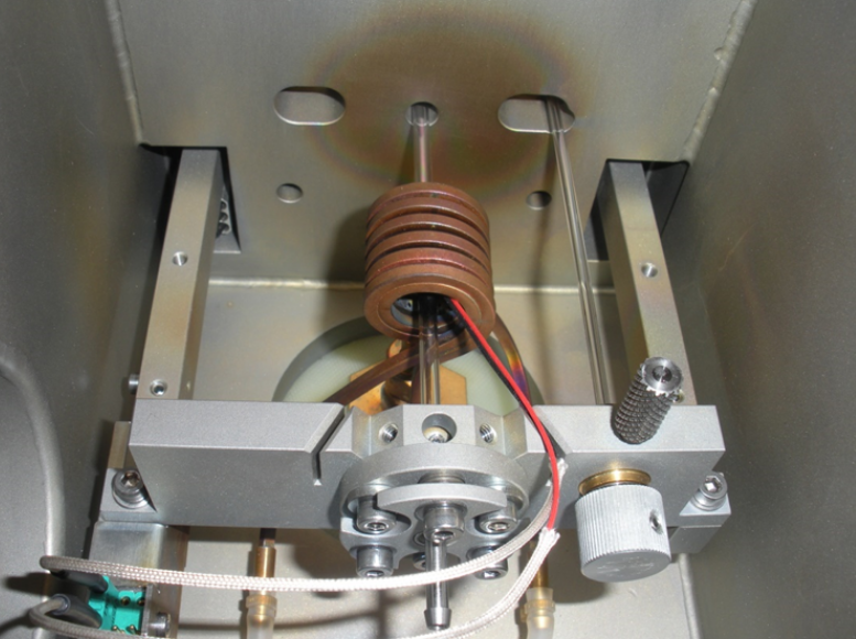
The goal of the computer models is to accurately predict the distributions of temperature in the sample during heating, holding, and cooling. The samples used in the test cell were 4 mm diameter by 10 mm long. The samples were held in place using fused silica tubes. A picture of the test cell is shown in Fig. 1. The specimen is suspended between spring loaded hollow fused silica tubes and a linear voltage displacement transducer is utilized to measure axial length changes. The unit is programmable such that linear heating and cooling rates can be attained within the limits of the power supply and quench capabilities. For this study, heating and holding were programmed followed by free quenching with helium.

In combination with the material tests, Fluxtrol, Inc. modeled the heating processes using Flux [4] software, while the cooling process was simulated by Airflow Sciences Corporation using the CFD programs Azore® [5] and ANSYS-Fluent [6] to understand the temperature distributions in the components. The reason for the modeling is to determine both the real temperature distributions and the “average” temperatures in the samples versus time, which can then be used to reinterpret and adjust the material behavior dynamics from the dilation measurements.

Figure 1: Quench dilatometer showing thermocouple leads, specimen suspended between fused silica tubes, outer water cooled induction coil, and inner gas quenching coil.

In an earlier paper by the authors [7], the effect of the current cooling system was analyzed, and it was determined that there were significant non-uniformities in the cooling rate along the length of the test specimen. The goal of the current work is to develop alternate cooling strategies that provide more uniform cooling and, if possible, faster cooling.

Assessment of Cooling Methods

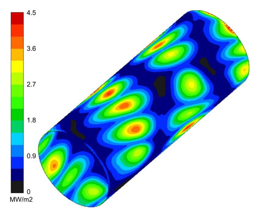
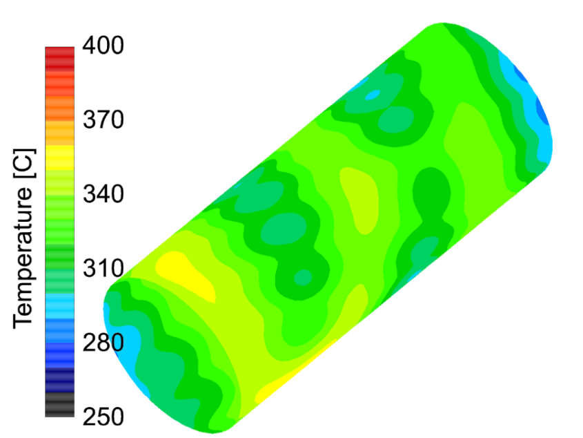
One of the motivations for this line of inquiry was a set of measurements that showed significant surface temperature variations between the near end, the center, and the far end of the dilatometry sample during the cooling process. The existing quench system consists of a helix coil bonded to the inside of the induction coil and featuring a series of small holes. CFD analysis of that system [7] confirmed the existence of variations in surface heat flux rate due to a combination of the pattern of holes in the cooling coil and the flow patterns created by the cooling jets. The predicted surface heat flux rates for that case are shown in Figure 2 while the surface temperature distribution 2.5 seconds into the cooling process is shown in Figure 3.

As a first step in the development of an improved cooling system, the effectiveness of several concepts to deliver convective cooling to the sample surface were evaluated using reduced domain models. All cooling concept CFD simulations were performed using Ansys-Fluent® [6]. The internal materials database was used for the transport properties of helium. Helium density followed the incompressible ideal gas law, thermal conductivity used a piece-wise linear relationship, while viscosity and specific heat were assumed to be constant over the range of helium temperatures expected.

Figure 2: Predicted surface heat flux during cooling for the existing helical coil quench. Figure 3: Predicted variation in surface temperature for the existing helical coil quench at 2.5s into quenching. Significant variations in temperature are seen.

Initial Cooling Concepts

One of the initial cooling concepts was to use axially aligned slot nozzles to direct flow tangent to the sample surface in order to create a swirling flow around the sample. Conceptually, this should provide a high degree of cooling uniformity. As shown in Figure 4 below, however, rather than creating a swirling flow around the sample, the jets tend to skim the surface and then diverge, in part due to the presence of the other jets. The level of heat transfer is also significantly lower than for the existing coil, which highlights the effectiveness of impinging flow for heat transfer applications.

Figure 4: The flow pattern resulting from axially aligned slot jets intended to promote swirling flow.

The next concept used the same slot nozzles, but directed them at the sample center, rather than directing them tangentially. The number of jets was varied to assess the effect on uniformity and overall cooling rate. Flow patterns for several options are shown in Figure 5.

The next concept used ring/slot jets that were spaced along the length of the sample. As shown in Figure 6, however, the convergence of the flow as it moves toward the surface of the sample created instabilities that distorted the jet sheet and caused it to divert away from the sample surface.

Figure 5: Assessment of different numbers of axial line jets for cooling the sample surface. Instabilities cause the jets to divert from the sample surface. Figure 6: Air from ring slot jet turns axially before reaching sample surface, leading to ineffective cooling.

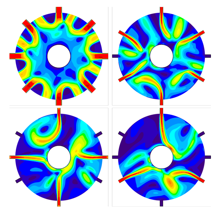
In order to alleviate this effect, the jet ring was divided into a series of individual slot jets arranged in a ring around the sample, as shown in Figure 7. This arrangement resulted in good stability of the jets and effective cooling.

A parametric study was performed to assess the effects of spacing between the jets and jet size on the overall cooling performance and efficiency. The results of that study are summarized in Table 1.

Figure 7: Flow field resulting from segmented ring slot. This arrangement is effective at bringing high velocity helium to the surface of the sample.

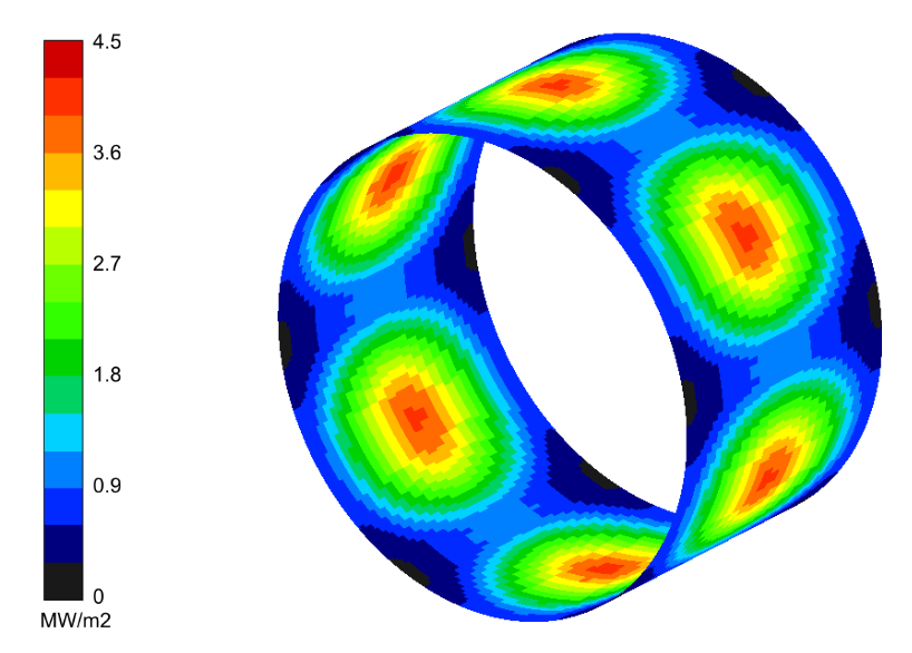
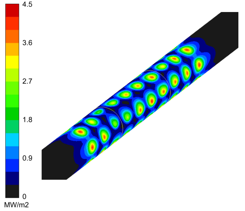
A spacing of 2.5mm between rows of nozzles was chosen to provide the best compromise of overall heat flux and efficiency of heat transfer. The heat flux distribution provided by a single ring of nozzles is shown in Figure 8.

Figure 8: Heat flux distribution provided by nozzles in ideal (symmetry) condition.

Impacts of Cooling System on Induction System

The existing helical quenching system is bonded to the induction coil and derives cooling from the water circulating through that channel. Implementation of the cooling system envisioned in the previous section requires helium delivery channels that are axially aligned, and must be electrically isolated from the induction coil. In order to prevent these channels from overheating during the induction phase of the test cycle, they will need their own set of cooling water channels. The presence of these copper channels within the cooling coil will have a negative effect on the induction system and the ability to heat the sample. An analysis was performed to assess these effects.

Model Development Strategy

3-D electromagnetic models using Flux software [4] were used to understand the current density distribution in the specimen. The material properties important for simulation were developed in a previous study [8].

To investigate the effect of the quench and cooling fingers on the current density of the specimen, two sets of models were made. The first model set included the fingers, while the other had no fingers, with everything else held constant. In addition, each set of models had cold steel and hot steel properties, at 900 °C, to investigate the effect of the fingers. Finally, 2-D models were made to compare to and validate the 3-D models.

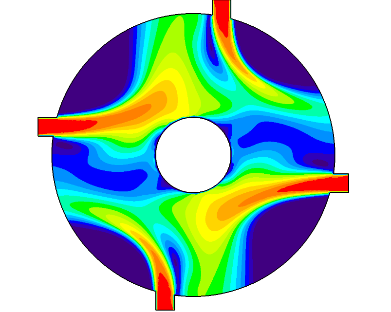
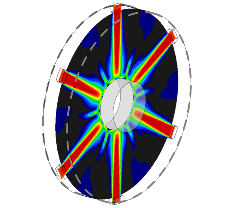
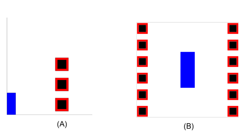
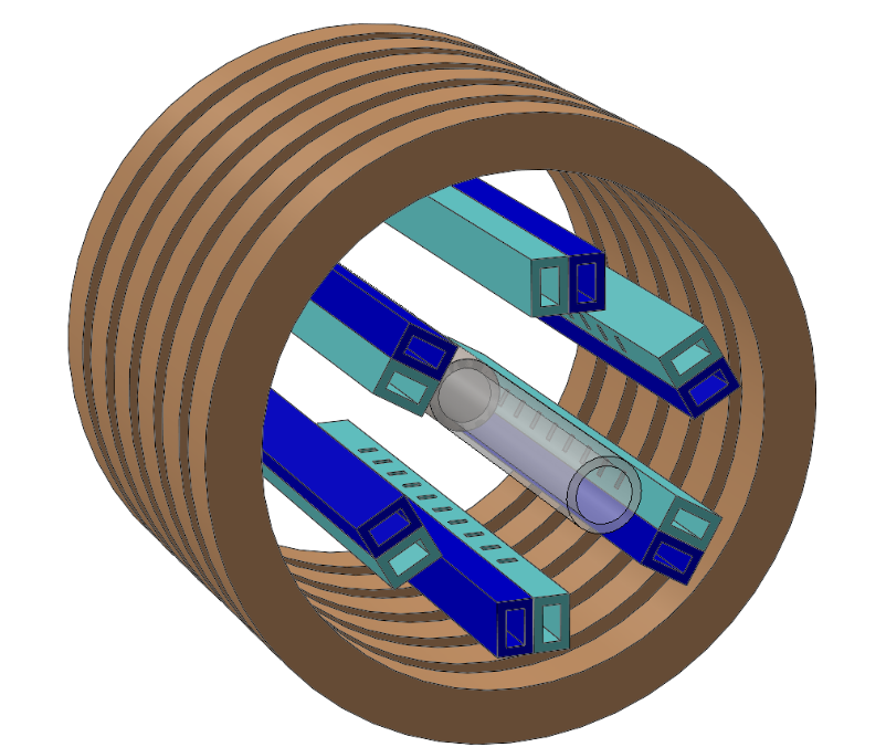
All models had a current source of 200 A at 240 kHz frequency. While actual current values will vary depending heating rate and specimen’s temperature, a constant current source was used for better comparison. To reduce the model’s size and cut the solve times symmetry planes were used, resulting in 1/12th of the 3-D system being modelled. Figure 9 shows the 3-D geometry used for the electromagnetic models.

Figure 9: (A) 1/12th of the 3-D geometry used for the electromagnetic model. (B) Full 3-D geometry of the electromagnetic model, shown by superimposing the partial geometry.

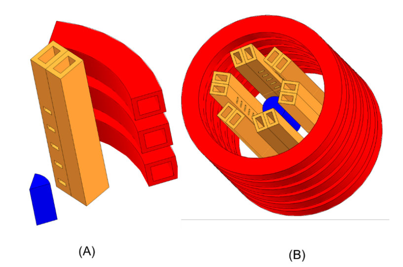
Figure 10 shows 2-D geometry used for the electromagnetic models. The 2-D models use axi-symmetric and half system symmetry.

Figure 10: (A) 1/2 of the 2-D geometry used for the electromagnetic model. (B) Full 2-D geometry of the electromagnetic model, shown by superimposing the partial geometry.

Results

The electromagnetic model results showed no significant difference in the current density distribution between the different cases. Figure 11 shows the specimen’s current density distribution for the 3-D and 2-D models of the cold steel.

Figure 11: Specimen’s current density distribution for all models using cold steel material properties. (A) 3-D model with cooling fingers, (B) 3-D model without cooling fingers, and (C) 2-D model without cooling fingers.

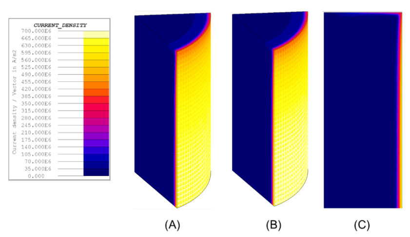
The results for the hot steel models showed no significant difference in the current density distribution between the different cases. Figure 12 shows the specimen’s axial surface current density distribution for the 3-D and 2-D models of the cold steel.

Figure 12: Specimen’s current density distribution for all models using hot steel material properties. (A) 3-D model with cooling fingers, (B) 3-D model without cooling fingers, and (C) 2-D model without cooling fingers

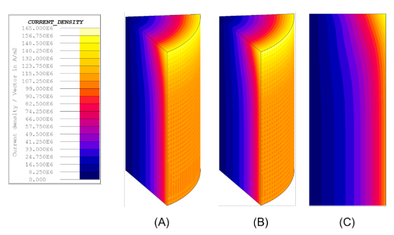
Figure 13 shows the graphs of the axial surface current density distribution for all the electromagnetic models.

Figure 13: Axial surface current density distribution graphs for all models.

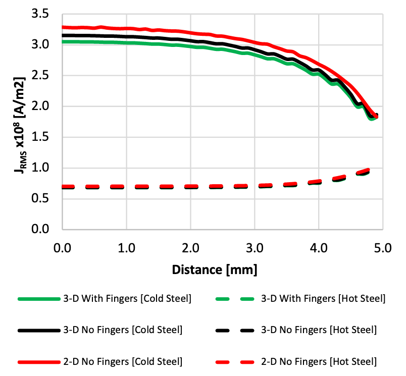
The results in Figure 13, along with the previous results, indicate that the current density is not significantly affected by the addition of the copper cooling fingers. The cold steel results show a higher difference in the current density than that of the hot steel values. However, the difference is not significant. Furthermore, the 2-D model results strongly agree with the 3-D model results.

Table 2 shows power and efficiency values for all models.

The results in Table 2 show no significant drop in the coil’s or specimen’s power with the addition of the cooling fingers. However, the addition of the cooling fingers adds a power loss source and increases the total required power, resulting in a reduced efficiency. The results show ~60% increase in the total power in cold steel case and a ~100% increase for the hot steel case. The results also show strong agreement between the 2-D and 3-D models.

The increase in total power due to the addition of the fingers means the dilatometry machine will not be able to run at the highest rated heating rates. Switching to a larger power supply will resolve the issue.

Cooling System Performance Analysis

Gas Flow Field

The cooling system developed using the reduced domain model was incorporated into a full 3D model. A rendering of that model is shown in Figure 14 below. A fully-structured grid was used to represent the geometry, using a total of 12.5 million computational cells.

Figure 14: System geometry. Brown – induction coil, turquoise – helium channels, blue – cooling channels.

The dilatometry chamber is evacuated during the heating cycle, such that the initial flow of gas will backfill the chamber to atmospheric pressure. Since the time needed to raise the pressure to ambient was calculated to be 0.011 seconds, that portion of the cycle can be safely ignored, with the flow field assumed to be steady-state for the bulk of the quenching operation.

The surface of the sample was held constant at the target temperature of 850 ºC for the quench chamber simulation. The simulation was run in ANSYS-Fluent® [6], and used the k-ω SST turbulence model to provide improved surface heat transfer predictions. The simulation required 10 hours to solve on a 3.0 GHz workstation using 32 computational cores.

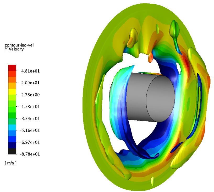
The flow field within this domain is shown in Figures 15, 16, and 17. Figures 15 and 16 show radial and axial planes through the domain, while Figure 17 shows a iso-surface of helium velocity, providing a comprehensive view of the density of impingement jets onto the sample surface. It should also be noted that there was some instability in the jets, with their trajectories wavering somewhat over time. While inclusion of this phenomena is outside the scope of the present research, it should be noted that such behavior would likely enhance the overall heat transfer rate.

Figure 15: Vertical slice through the computational domain showing the impingement of helium on the sample and fused silica tubes. Only two jets are in the plane of this cut (lower portion of coil, either end). Figure 16: End view showing helium jets impinging on the sample. Figure 17: Isometric view of sample with isocontours of helium jet velocity (surface velocity = 75 m/s). Colors relate to the tangential velocity component. Central section is the sample, while the outer sections are the quartz rods.

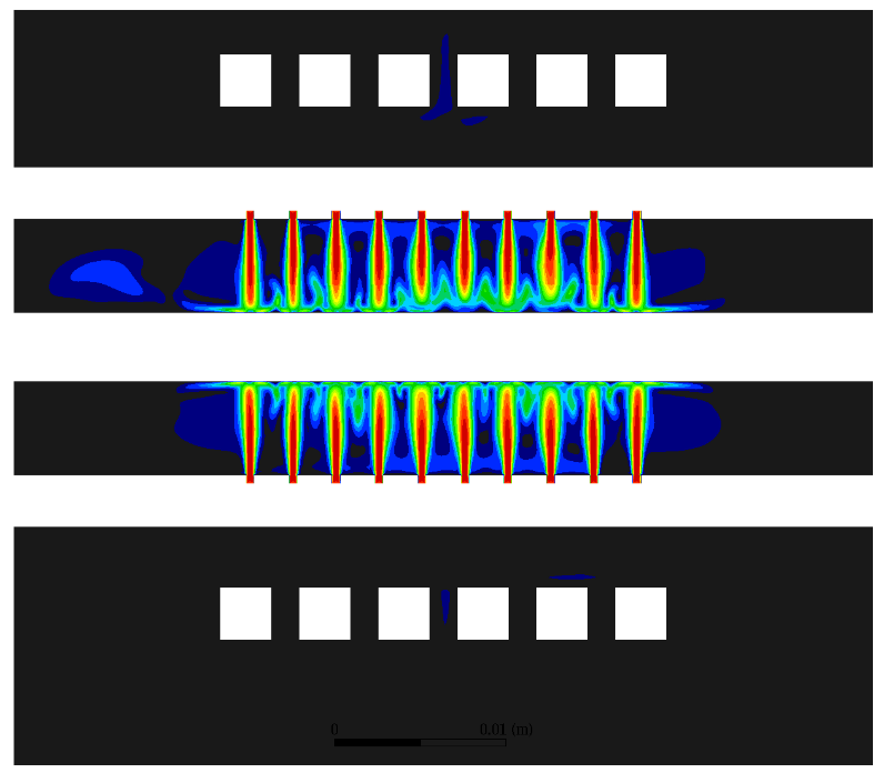
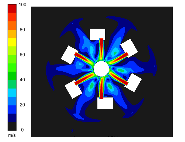
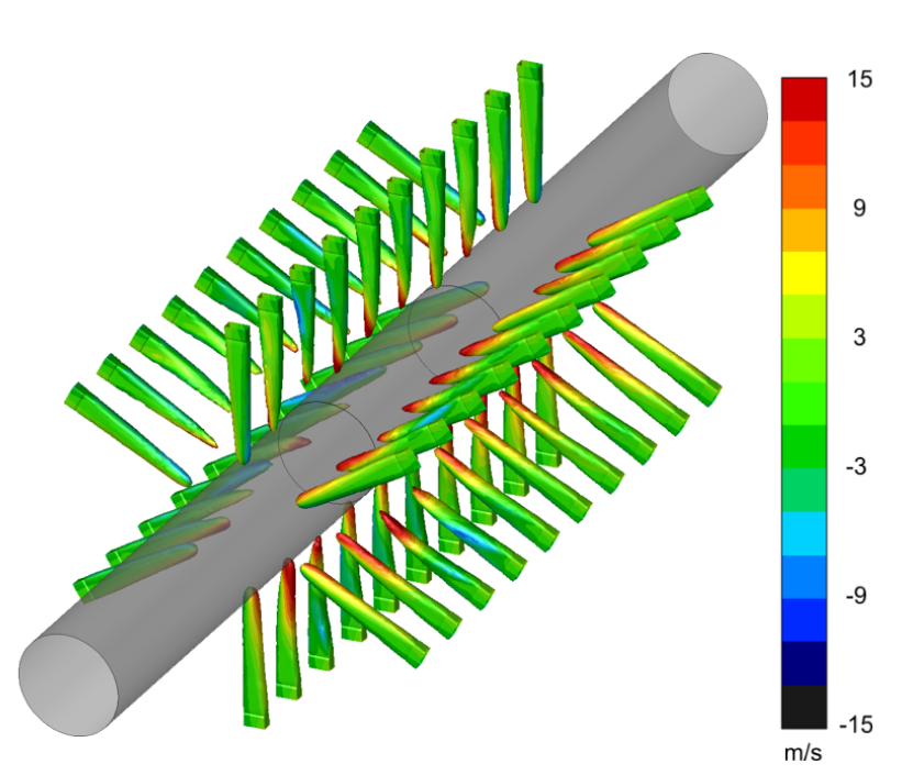
Figure 18 shows the surface heat flux distribution on the sample surface. Is should be noted that there are significant differences in the heat flux rates between the impingement locations and the balance of the sample surface. This variation could mean that the measured surface temperature could be very sensitive to the placement of the thermocouples, with placement under a jet showing faster cooling than adjacent areas.

Figure 18: Surface heat flux distribution, showing the effect of jet impingement on heat transfer. The length of the sample is delineated by white lines.

Sample Cooling Prediction

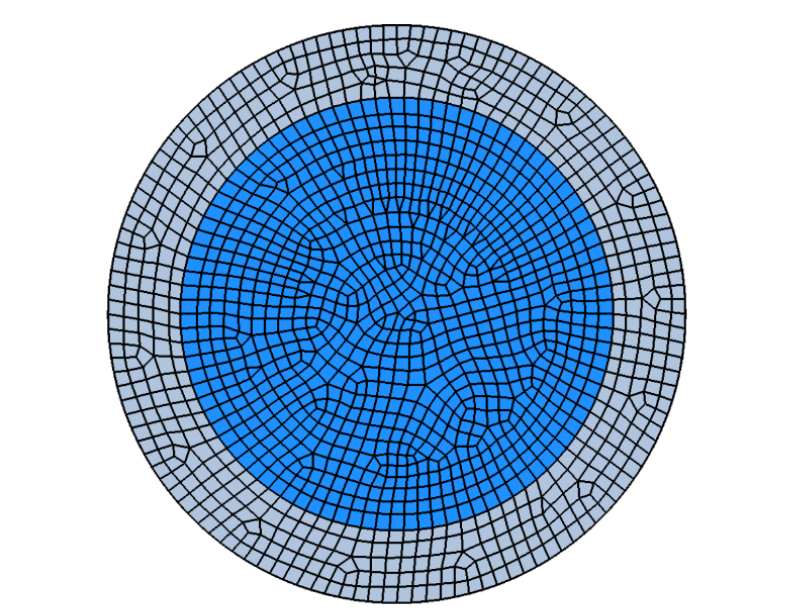
Surface heat flux rates from this model were then converted to surface heat transfer coefficients and applied to a CFD model of the sample and fused silica tubes. Note that there were no fluid domains in this model. In addition to the convective heat transfer coefficient, radiation from the surface to ambient surroundings was also included in the simulation. A view of the computational domain and grid is shown in Figure 19. A total of 320,000 cells were used for this model.

Figure 19: End view of the computational grid for the thermal model, including the fused silica tube (gray) and the sample (blue).

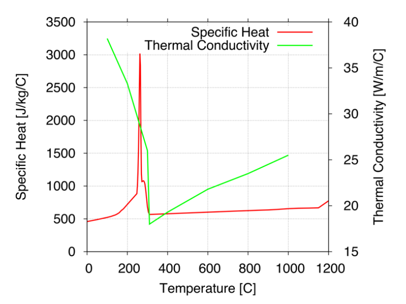
The specific heat and thermal conductivity curves used for the O1 steel in the cooling simulation are shown in Figure 20. The Cp curve at high temperatures follows typical data for Austenite, while the phase change excursion in the Cp values is shifted to lower than typical temperatures in accordance with the thermocouple data. The shape of that excursion was taken from DSC data collected for C-30Mod steel [9], which had a heat of phase transformation of about 84 J/g. The curve was further modified to reduce the latent heat amount to around 57 J/g in order to provide a better match with the observed data. Following this heat treatment cycle, the O1 tool steel is expected to have about 20% retained austenite, which may help to explain the lower heat of transformation. These adjustments may reflect not only the material but also the processing conditions, such that this Cp curve may only be applicable to this situation.

The thermal conductivity curve followed values typical of Austenite down to the start of Martensite transformation and rises to values typical of ferrite through the transformation period.

Figure 20: Specific heat and thermal conductivity curves used for thermal simulation of O1 steel.

As with the previous study of dilatometer quench cooling [7], the heat flux rates provided by the CFD simulation were increased by 28%, as it was shown that doing so would provide a better match to the data. The cause of this discrepancy is not known.

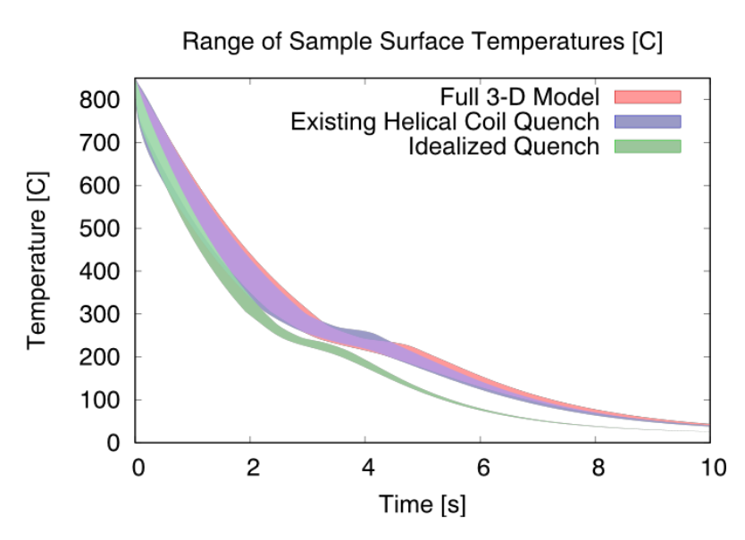
Simulations of the sample cooling were performed for two different cases – the ideal case represented by the reduced domain model and represented by the heat flux distribution in Figure 8 and the heat flux distribution from the full 3D case, as shown in Figure 18. While the full 3D case should provide the same distribution as the ideal case, instabilities in the jets, as shown in Figure 17, result in a reduction in the overall heat flux rate. While the ideal case scaled heat flux is 1.92 MW/m^2, the full 3D case has a scaled average heat flux rate of 1.46 MW/m^2.

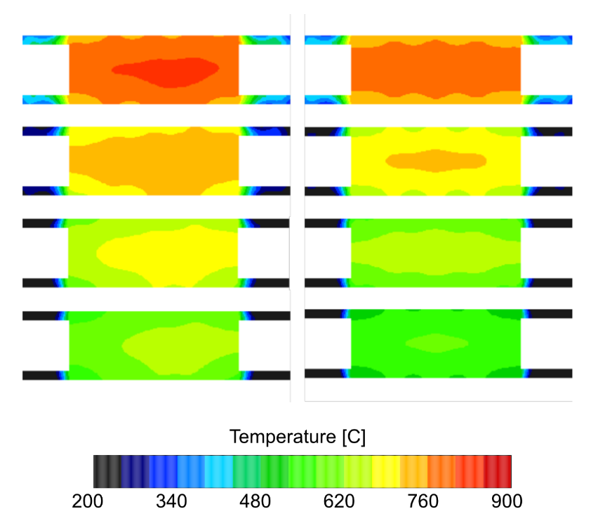
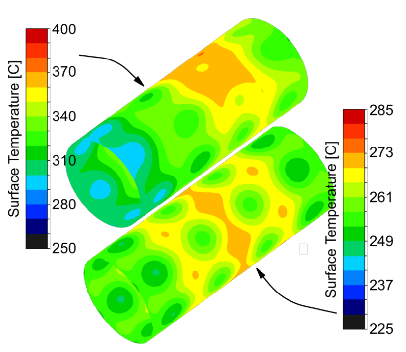
The predicted temperature profiles under these modified boundary conditions for slices through the sample geometry are shown in Figure 21 for several different moments in time, while an isometric view of the surface temperature is shown in Figure 22.

A comparison between the surface temperature history for the existing coil quench, modified coil quench, and idealized modified quench is shown in Figure 23. While the idealized case shows faster cooling and a tighter distribution, the results for the full 3D case are not significantly different than for the existing helical quench. The reduction in performance between the idealized case and the actual model results reflects the instability of the helium jets. Thus, achieving improved quenching performance requires the development of stabilizing the jets in a practical and effective manner.

Figure 21: Temperature distribution in vertical slice through sample and fused silica tube at 0.25, 0.5, 0.75, and 1.00 seconds into quenching process. Left is full 3D model, right is ideal case. Figure 22: Surface temperature distribution 2.5 seconds into quench cycle. Upper image is for full 3-D case, while lower image reflects the ideal case. Note the different temperature scales, reflecting the difference in average heat flux between the two cases. Figure 23: Comparison between measured thermocouple values and CFD predicted min, max, and average surface temperatures.

Summary

This paper investigated methods of improving the quench uniformity and rate for the TA Instruments DIL805 dilatometer. Previous papers by the authors demonstrated that measured variations in measured surface temperature during the quench portion of the operation were due to the flow dynamics of the helium jets emanating from the helical quench coil.

Several alternate quench concepts were investigated to provide higher and more uniform quenching rates. Many of the concepts failed at the early stage of investigation, as the flow dynamics were shown to be highly unstable and provide low heat flux rates. The best method appeared to be a series of individual jets, not unlike the current helical coil system (though the pattern was somewhat different). While delivering high velocity gas to the sample surface is key to providing high heat flux, there also needs to be a pathway for the gas to flow away from the sample.

The chosen method for further investigation featured supply tubes axially aligned with the sample with rows of holes. In order to maintain the temperature of those tubes at reasonable levels during the induction heating portion of the cycle, cooling tubes would also be needed. The effect of these structures on the induction system needed to be assessed.

The electromagnetic models show the addition of the cooling fingers has no significant effect on the current density distribution, and as a result power density distribution and heating. The models also show that the there is a significant drop in efficiency due to losses induced in the cooling fingers. The updated quench design will not affect the induction heating portion of this process. But the reduced efficiency will require an increased power source to maintain the higher heating rates.

A full 3D model implementation of the cooling system was modeled in CFD, and the surface heat flux rates were extracted. The previous CFD study by the authors showed that the CFD-predicted heat flux rates were 28% lower than those indicated by experimental measurements. The reason for the discrepancy is not known.

The full 3D model showed heat flux rates and uniformity that were not as good as the idealized case used to develop the flow dynamics using a smaller, periodic domain model. The reduction is due to the flow dynamics and interactions between the individual jets.

Analysis of the sample cooling rate showed that while the cooling concept provided increased cooling rates and better uniformity, the actual performance predicted by the full 3D model was no better than the current quench method. Additional study would be needed to develop systems of jets that were more inherently stable in order to realize the goal of improved cooling.

Acknowledgements

The authors acknowledge the support of Airflow Sciences Corporation, Fluxtrol, Inc. and the corporate sponsors of the Advanced Steel Processing and Products Research Center, an industry/university cooperative research center at the Colorado School of Mines.

References

[1] Clarke, K. D., and Van Tyne, C. J., The Effect of Heating Rate and Prior Microstructure on Austenitization Kinetics of 5150 Hot-Rolled and Quenched and Tempered Steel, Proceedings of MS&T 2007, September, 2007.

[2] Cryderman, R. L. and Speer, J. “Microstructure and Notched Fracture Resistance of 0.56% C Steels After Simulated Induction Hardening,” Proc., 29th ASM Heat Treating Society Conference, Oct 24-26, 2017, Columbus, Ohio.

[3] Fukuzawa, K.,Misaka, Y., and Kawasaki, K.,, “The Effects of Grain Refinement on the Fatigue Properties of Induction Hardened Cr-Mo Steel,” Proc., 17th IFHTSE Congress, Oct 27-30, 2008, Kobe, Japan.

[4] Altair, “Hyperworks,” www.altairhyperworks.com

[5] Azore Software, “Azore®” , www.azorecfd.com

[6] ANSYS-Fluent, www.ansys.com/products/fluids/ansysfluent

[7] Eddir, et. Al.., “Influence of Heating Rates on Temperature Gradients in Short Time Dilatometry Testing”, Thermal Processing in Motion Conference, June 5-7 2018, Spartansburg, South Carolina, USA

[8] Goldstein, R., Buchner, E., and Cryderman, R., “Modeling of Short Time Dilatometry Testing of High Carbon Steels”, Proceedings of the 29th ASM Heat Treating Society Conference, October 24–26, 2017, Columbus, Ohio, USA

[9] Taylor, R., Groot, H., and Ferrier, J., Specific Heat and Heat of Eutectoid Transformation of C38-Mod Microalloy Steel, Thermophyical Properties Research Laboratory, Purdue University, 1995.

If you have more questions, require service or just need general information, we are here to help.

Our knowledgeable Customer Service team is available during business hours to answer your questions in regard to Fluxtrol product, pricing, ordering and other information. If you have technical questions about induction heating, material properties, our engineering and educational services, please contact our experts by phone, e-mail or mail.

Fluxtrol Inc.
1388 Atlantic Boulevard,
Auburn Hills, MI 48326
Telephone: +1-800-224-5522
Outside USA: 1-248-393-2000
FAX: +1-248-393-0277

Related Topics

• ASM HTS 2019 Improving Corrosion Resistance of Soft Magnetic Composites for Induction Heat Treating Applications
• ASM HTS 2019 Improving Inductive Welding System Performance with Soft Magnetic Composites
• Modeling of Short Time Dilatometry Testing of High Carbon Steels
• Influence of Heating Rates on Temperature Gradients in Short Time Dilatometry Testing