Information
Authors: Prem P. Vaishnava, Robert C. Goldstein
Location/Venue: HES 19 Padova, Italy
Download Presentation PDF
Abstract
Many induction heating coils use soft magnetic composite materials (SMCs) to improve induction system performance. In demanding induction heating applications, the core loss in the soft magnetic composite material is one of the critical factors in predicting the reliability of the induction coil using computer modelling. In this paper we have used calorimetry method for experimentally determining core losses in SMCs up to ≈1 T magnetic flux densities at a frequency near 150 kHz. This paper contains a discussion on the limitations of current methods for calculating core losses. To address these limitations, a new method for calculating core losses is presented. Using the new method, the results of the core loss measurement did not fit well with traditional core loss models over the full range of magnetic flux densities. A discussion on the different models and a hypothesis for the source of the variation from the models is presented.
Introduction
SMCs are used on many different types of induction heating coils. One of the important factors in the design and optimization of a reliable induction heating coil is the accurate calculation of power losses in the soft magnetic composite materials. In order to properly model induction coils with SMCs, it is critical to understand the magnetic core loss behavior over the entire operating range of induction heating conditions.
The source of heat generation or the magnetic core loss in SMCs can be divided into two main categories: Hysteresis losses (h) and eddy current losses. The eddy current losses can be further divided into individual particle eddy current losses (ipe), local eddy current losses (local) and global eddy current losses (global). The total power loss is the sum of these losses [1].

For proper characterization of a magnetic material, it is desirable to make a measurement of the non-geometry dependent components of core loss (hysteresis and individual particle eddy currents). Computer modeling software is appropriate for calculation of local eddy currents and global eddy currents in the core used on an induction heating coil. For many decades, empirical equations have been used to statistically fit the experimental data to provide estimates of core losses in the materials. In 1892, Steinmetz [2] proposed an equation to fit power loss with magnetic field, given by

where Pv is the power loss per unit volume, B is the maximum peak flux amplitude, β and k are curve fitted coefficient obtained from experiment. The original Steinmetz equation did not include frequency and calculated the core loss per unit volume of the material. Later, to increase the accuracy of the estimation, more terms were introduced in the equation.
Modified Steinmetz’s equation, also known as the Power Law equation, that incorporates frequency, is the standard core loss equation that is used by many manufacturers, scientists and engineers. Power law equation is given by

Where Pv is the power loss per unit volume, B is the maximum flux density and f is the frequency. k, a, b are the parameters that are determined by actual experimental data for a given material. Generally, the modified Steinmetz equation will work well over a limited range of field strengths and frequencies.
More recently, a new model has been proposed by Bertotti, et. al, [3] which attempts to better describe the losses by breaking them down into individual components. The Bertotti’s model equation is as follows [3]

In the equation (4), f and B are the frequency and the maximum flux density; 𝑘hy,eddy, 𝑘ex and 𝑏 are the material specific parameters determined by curve fitting experimental results. The three components of loss in the model are hysteresis, individual particle eddy current and “excess” losses (other losses). Hysteresis loss is first order in frequency. SMCs are designed for use in frequency ranges where individual particle diameter is significantly less than the reference depth of the particle. Therefore, individual particle eddy current heating should be proportional to the square of frequency and magnetic flux density in the particle at a given temperature. Magnetic cores for testing are sized such that global and regional eddy currents are negligible. The “excess” loss is a curve fitting tool to account for losses being higher than trend at low fields.
Eggers, et. al [4] observed that the Bertotti model had the following limitations i) assuming linear material behavior where the permeability is constant near the operating point and ii) proposed a rule of thumb that the equation is valid for flux density value B ≤ 1.2 T and frequencies f ≤ 400 kHz.[4]. Eggers et al, along with some other groups, proposed additional correction factors for their model. However, in the end the authors found that the practically all models have very limited applicability to soft magnetic composites used under the full range of induction heating conditions which can operate at flux densities of mT up to over 1T at frequencies from 15-20 kHz up to a few MHz
For proper modeling heat generation within SMCs for induction heating, it is desirable to have an equation that can cover the full range of conditions that a magnetic core could be used in. To have the proper description, it is necessary to think of the material as a sum of discrete magnetic particles, rather than a single homogenous material. Therefore, the magnetic core loss for a core with n particles should be described as

With Pcore being the total power in the core and Pi being the power in the individual particle. The power in any given particle can be accurately described by

Which can be expanded to

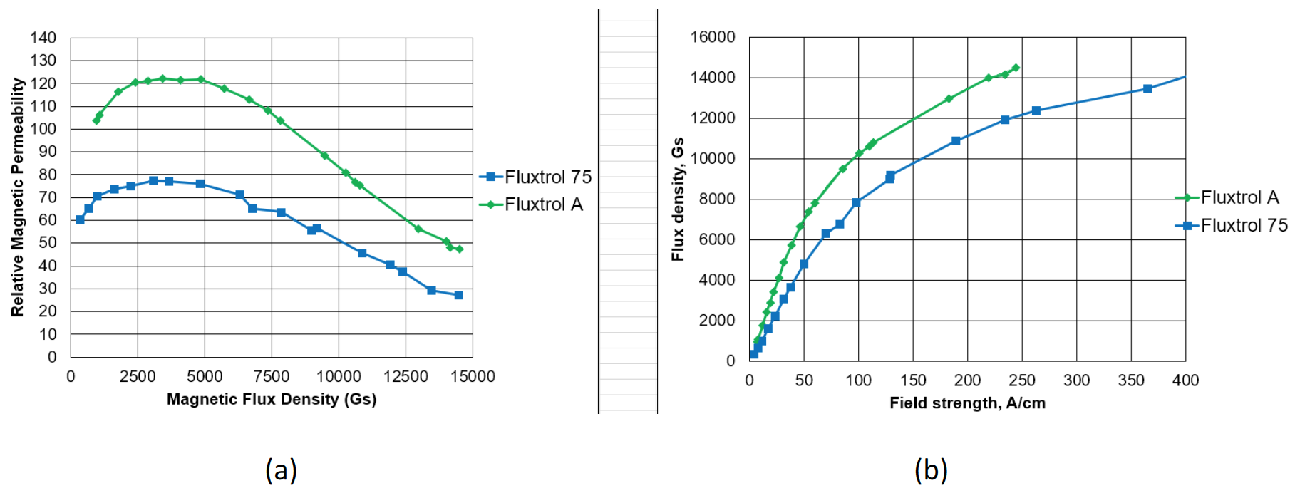
Because SMC’s are inhomogeneous and consist of a distribution of particle sizes separated by varying thicknesses of non-magnetic materials, there are multiple potential parallel paths in the magnetic circuit. This leads to a magnetic flux density distribution that is not homogenous on the microscopic level within the cross-section of the core and different particles are at different flux density levels. The distribution of the flux density levels can explain the quasilinear behavior of SMCs and why it is very difficult to fully saturate them (Figure 1). Flux in these non-magnetic regions between particles does not generate additional loss (hysteresis or eddy current) in the core. Flux in the magnetic regions does generate loss in the core. Therefore, as magnetic permeability of the bulk material increases, or decreases the percentage of magnetic flux flowing in magnetic particles and generating magnetic loss increases or decreases.
As we get to very high fields, the preferred paths are already saturated and lesser magnetic paths take greater percentages of magnetic flux. With little change in magnetic flux in the individual particle, there is very little change in the loss in that individual particle. Because all of the flux paths are broken by non-magnetic materials at multiple points, the differential in reluctance between the magnetic paths and the airgaps in parallel, becomes smaller and smaller meaning more and more of the additional flux is not actually flowing in the particles, but in the non-magnetic materials separating them.
Finally, as the permeability of the particle varies, the eddy current component of the loss should vary as the ratio of the particle diameter to the reference depth changes. Therefore, the proper description of both sources of loss needs to have a component that is proportional to the magnetic permeability of the core, which may not be the same.
In this paper, magnetic losses at frequency close to 150 kHz and magnetic flux densities up to and exceeding 1 T were measured and compared for two commercially available soft magnetic composites, Fluxtrol A and Fluxtrol 75. The losses were measured by calorimetric method. Although the calorimeter used was insulted from the surroundings, it was found that it was losing a significant amount of energy to the environment that was having an impact upon the measurement results. Efforts were made to understand and quantify this loss and incorporate it into a new calculation method. For the new method, temperature was measured at multiple key points in the system to provide information on the thermal gradients within the system. Power loss to the environment was adjusted for each data point and calculated from the cooling data.
Experimental and Core Loss Determination Method
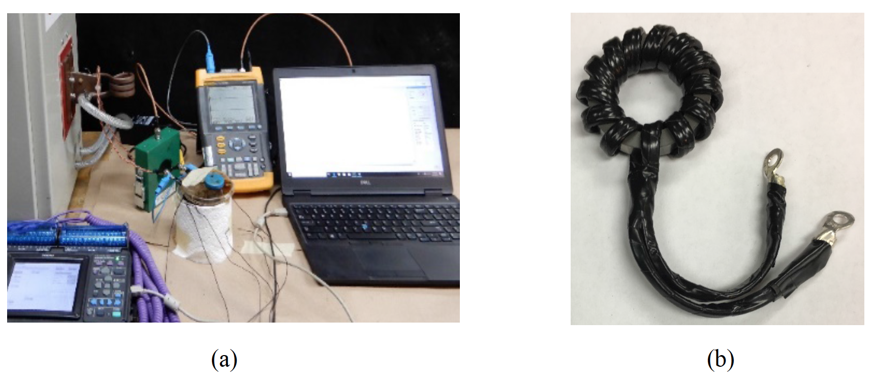
The losses were measured by calorimetric method where the toroid of the material was wrapped with litz wire and immersed in a high boiling point liquid (Figure 2a). A 25 kW 135 – 400 kHz power supply was used for the testing. The power supply had a 3 turn coil water cooled coil connected to the front of the unit with a relatively small inductance for tuning purposes. The toroidal core (shown in Figure 2b) was connected in parallel with the 3 turn coil. The generator output display voltage between 150 Vrms (approximate minimum power of unit) and 500 Vrms (maximum output voltage) was used with a given toroid and winding for the trials. Measurements were taken at various voltages in this range for a given winding. Once the maximum voltage level was reached, the number of turns on the core was reduced strategically so that additional trials could be conducted at a range of flux densities below the maximum from the previous turns number and significantly above that number. Voltage was measured close to the winding and efforts were made to minimize the inductance loss between the measurement point and the winding of the core. The overlap in readings assures that there is continuity between measurements with cores with different turns numbers. Flux density magnitude was calculated based upon the measurement of the mean RMS voltage in the coil and multiplying this value by the root square of 2. The reasoning behind this method as opposed to calculating from the magnitude of voltage are included in the results discussion section.
1-3 litz cables in parallel depending upon the number of turns were used to keep winding resistive loss low compared to the core loss and maximize the percentage of the core under the windings to try to maintain as uniform as possible core loading azimuthally at high flux densities close to saturation. Finally, the windings were made flat and parallel in order to maximize the percentage of the cross-section filled by toroid to minimize error induced by bypass flux flowing in the airgap between the core and winding (Figure 2b).
The high boiling point liquid was used to remove error associated with phase change and conservation of mass from the loss evaluation. It has been the authors experience in similar trials that the core temperature is significantly higher than the bulk fluid when testing and condensation of water vapor has been visualized on the lid of the calorimeter and steam has been emitted from the liquid during some trials.
In our previous trials, the individual test error was high (over 100%) based upon repetitive testing. Investigation into this error revealed that there were two main sources of error in the trials – loss to the environment and significant thermal gradients within the fluid. Although the calorimeter used was insulted from the surroundings, it was found that it was losing a significant amount of energy to the environment that was having an impact upon the measurement results, especially at low magnetic loss levels.
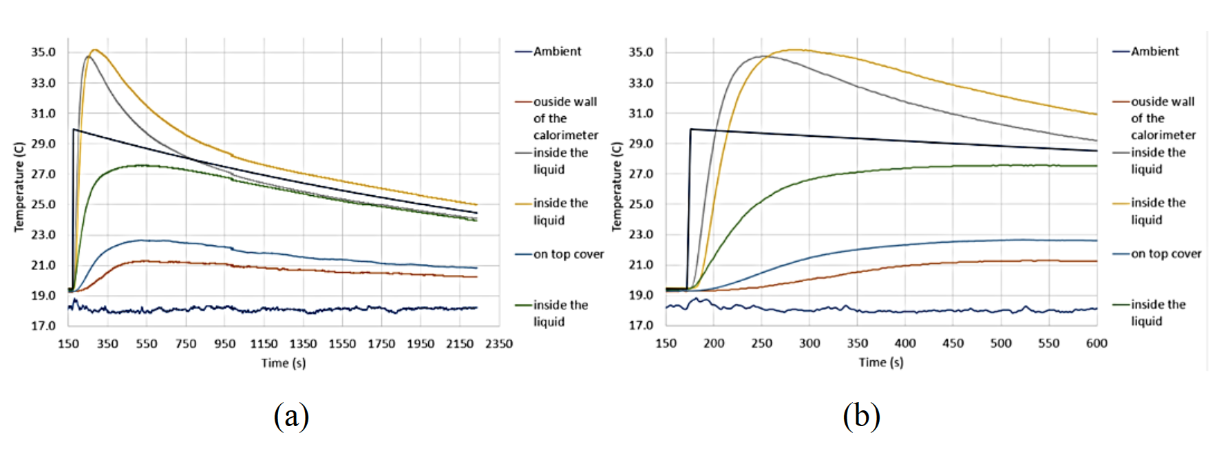
Existing methods used for core loss calculation, such as the initial slope method, greatly underestimate core loss amounts due to thermal lag in the system and therefore could not accurately determine the fluid temperature and the exchange of heat from the environment. Other methods, such as simple calorimetric calculation based upon fluid temperature rise divided by heating time, may over or under estimate the core loss based upon thermocouple location. To improve the accuracy of our calculations, temperature was measured at multiple key points (three places inside the liquid, one on the outside surface of the calorimeter, one on top of the lid and one ambient temperature) in the system to provide multiple data points for the analysis. The energy deposited in the core was averaged over the volume of the fluid, core, winding and inner calorimeter and applied to the volume for the time recorded in the trial. Losses from the inner calorimeter were calculated at each step in the process and subtracted from the energy deposited in the core at a given time during heating and cooling. Power loss to the environment was adjusted for each trial and adjusted to match the mean temperature of the fluid from the cooling data once the fluid temperature had reached quasi-equilibrium conditions. The temperature curves for a representative case are presented in Figure 3. It can be seen in this data that the difference in simple calorimetric calculations for the lowest thermocouple reading and highest thermocouple reading would be close to 100% based upon the difference in delta T values (approximately 8 C vs approximately 16 C). Flux density magnitude was calculated based upon the measurement of the “RMS Voltage” in the coil and multiplying this value by the root square of 2. The reasoning behind this method as opposed to calculating from the magnitude of voltage are included in the results discussion section.
Test Results and Discussion
Trials were run for Fluxtrol A and Fluxtrol 75 (Figure 4). The maximum magnitude of flux density achieved for Fluxtrol A was just under 1.2 T and for Fluxtrol 75, just over 1 T. The frequencies for the individual trials varied between 156 and 161 kHz. The power density values are normalized to 150 kHz based upon an assumption of losses being directly proportional to frequency. We were unable to achieve higher flux density levels during these trials due to the generator response to the operating conditions.
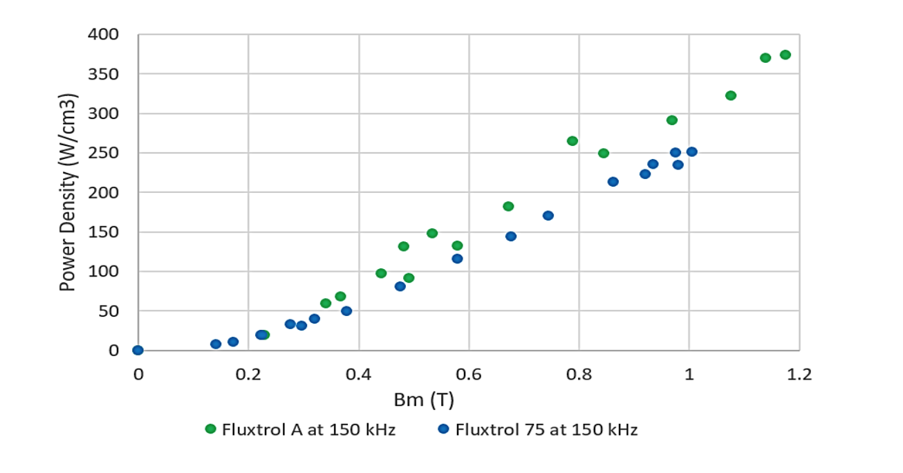
From the curves above, the losses for Fluxtrol A are somewhat higher than Fluxtrol 75 over the flux densities tested. To make a more detailed analysis of the behaviour, it is necessary to isolate the curves and review the data over a narrow range of magnetic permeabilities. If we look magnetic permeability curves for Fluxtrol A and Fluxtrol 75 (Figure 1) we can see that between 0.15 and 0.6 T flux density values, the permeability curves are approximately flat and close to their maximum value. Over this range, the data fits very well to the Steinmetz model with an exponent for flux density of 2.0. For both curves, the data point 0, 0 was used as core losses are 0 at 0 flux density (Figure 5).
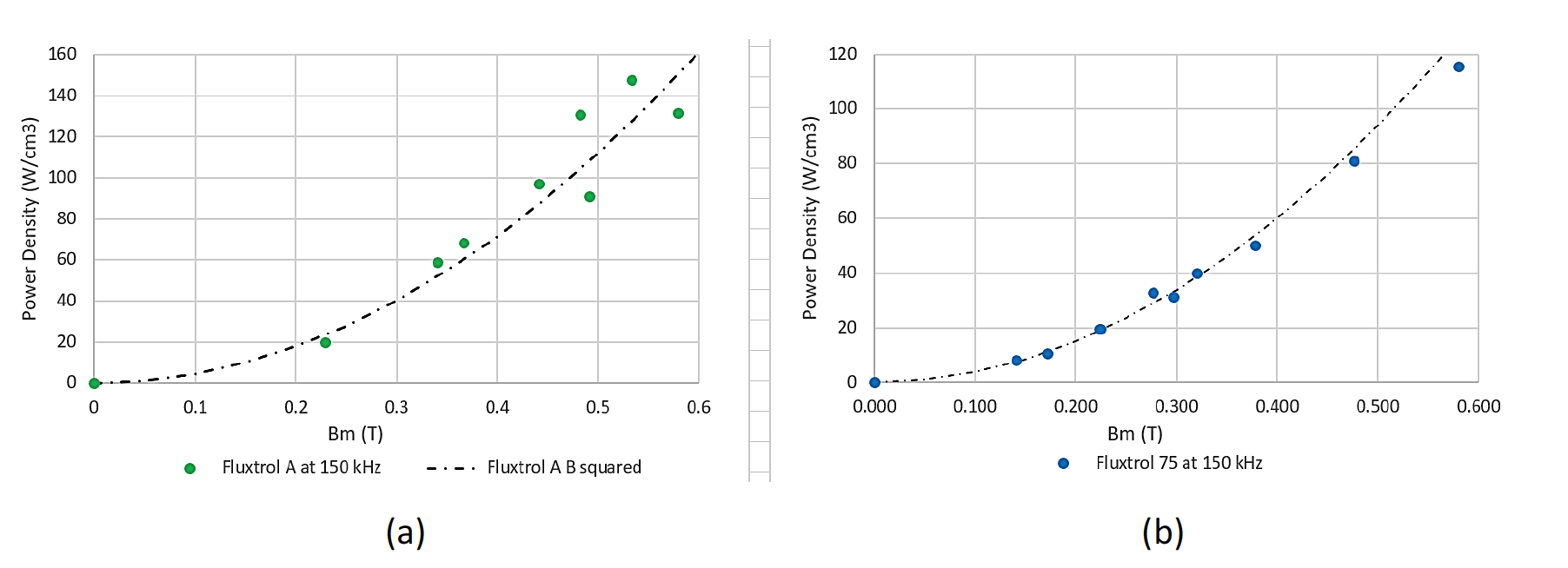
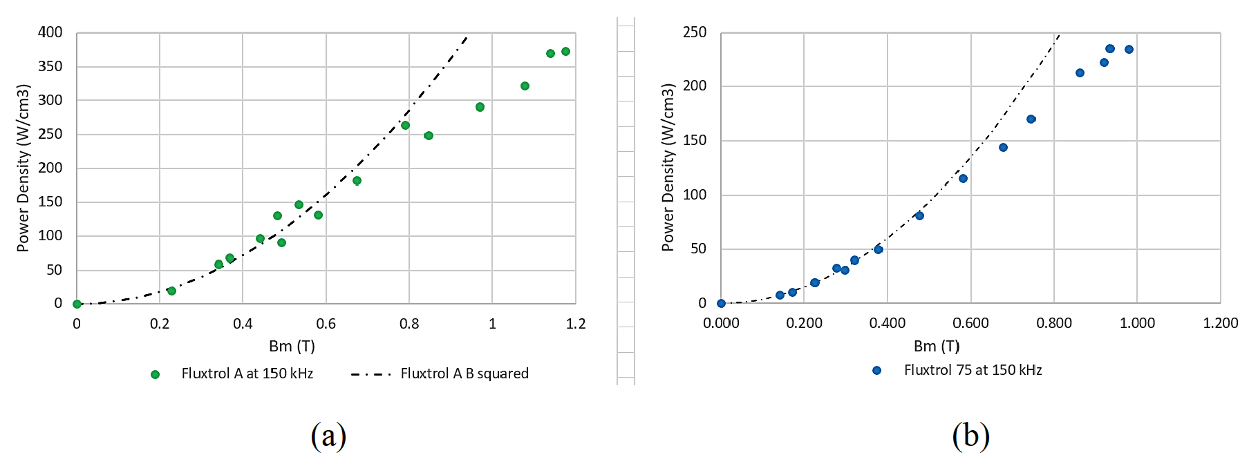
Figure 6 shows the same curves and Steinmetz model, but with data up to the maximum flux density level tested for the material. Above 0.6 T, the power loss values begin to diverge from the flux density squared approximation. The higher the level of magnetic flux, the greater the divergence from the curve. In addition, there is some evidence that the curves are beginning to plateau.
As noted above, the value of the magnitude of flux density used for the correlations is calculated from the mean rms value of the voltage. The reason for this is the main use of the data we generate is for calculation of losses in cores for induction coil component temperature prediction using computer simulation. In most commercial induction heating modelling software used for the heating process simulation, the calculations are done in the frequency domain rather than the time domain. This means that the voltage is approximated to have a sinusoidal waveform.
As flux density increases and a magnetic core approaches saturation, the shape of the waveform in our trials goes from a sinusoidal wave to triangular wave to progressively larger levels of distorted wave form (Figure 7 a). In this case, the ratio of the magnitude of voltage to the rms value of voltage increases to values larger than the root square of 2. This means that the magnitude of flux density is higher. However, since the software will inherently assume the relationship is sinusoidal, it means that the model will underestimate core losses, leading to a lower predicted value of temperature in the SMC than will occur. By calculating the magnitude of flux density from the rms voltage, the core losses in the models will better correspond to real performance conditions.
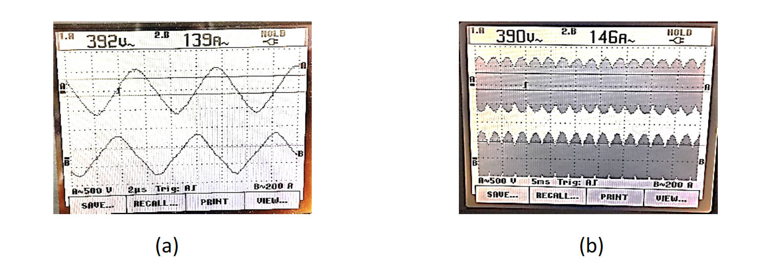
In addition, in most induction heating applications, there is not a true constant sinusoidal voltage applied. Usually, there is some oscillation of the magnitude of the voltage due to imperfect rectification of the line frequency voltage (Figure 7 b). This means that the rms voltage value will be varying in time at a much lower frequency than the process is operating at (except for the processes in the 100’s of Hz). To compensate for this, the scope is set to a long-time division (5 ms) when calculating rms voltages, hence the term “average rms voltage” is used for convention in the data. Most computer models do not consider this effect, so the authors feel this is the best value to use at the current time for calculations.
Conclusions and Future Work
Many induction heating coils use soft magnetic composite materials (SMCs) to improve induction system performance and these materials perform under a wide variety of conditions. In order to improve the ability to accurately model induction coil performance, it is necessary to provide improved material properties data.
We reviewed the literature on test methods for magnetic core loss measurement using a calorimetric method. Initial testing revealed very high levels of error and poor test repeatability. A detailed analysis was performed on the test system and it was found that there are three main sources of error in the methods, phase change/conservation of mass in the fluid, thermal lag in the system, and thermal loss to the environment. Solutions were presented to address these issues including the use of a high boiling point liquid, multi-point temperature measurement and a method involving averaged thermal body temperature calculation with dynamic thermal loss calculation based upon cooling curve analysis.
Using this method, we presented core loss results for two commercially available SMC’s, Fluxtrol A and Fluxtrol 75, at magnetic flux densities between 0.1 and 1.2T at frequencies between 156 and 161 kHz. The data were normalized to 150 kHz. The data fit very well to a flux density squared relationship, up to 0.6 T when the magnetic permeability of the core was relatively constant. Once the magnetic permeability started declining with increasing levels of flux density, the flux density squared relationship significantly overestimated the level of core loss. As the flux density increased further to values closer to the saturation flux density, the divergence increased, and the values of core loss appeared to be starting to approach asymptotically a threshold value.
The proposed hypothesis for this behavior is due a combination of magnetic saturation and the natural inhomogeneity of SMC materials. SMC’s consist of a combination of magnetic particles and non-magnetic materials separating them. This leads to multiple parallel magnetic circuits, some very efficient and some less efficient. As the permeability of an individual magnetic particle in a magnetic circuit declines approaching saturation, the efficiency of the magnetic circuit also declines, leading to additional magnetic flux flowing in less efficient magnetic circuits, which inherently have more non-magnetic space and less high magnetic permeability paths. Magnetic core losses (except for global eddy currents) will only occur in the magnetic materials in the circuit. Therefore, more and more of the additional flux in the SMC is in components that will not heat when exposed to an alternating magnetic field. Once all the magnetic particles are fully saturated, then a threshold value of core loss should be achieved.
Additional measurements are planned to use all commercially available material grades of Fluxtrol and Ferrotron products at multiple frequencies between several kHz and several hundred kHz. Once all the data is assembled, efforts will be made to create a correlation that accurately fits all the data studied. This information is expected to be available in the summer of 2019.
References
[1] Goldstein, R.C. (2014). Magnetic Flux Controllers in Induction Heating and Melting. ASM Handbook Volume 4C, 633-645.
[2] C. Steinmetz, On the law of hysteresis, AIEE Transactions, vol 9, pp 3-64 (1892).
[3] G. Bertotti, General Properties of Power losses in soft ferromagnetic materials, IEE Trans. On Magn., 24, 621-630 (1998).
[4] D. Eggers, S. Steentjes, K. Hameyer, Advanced Iron-Loss Estimation for Non-Linear Material Behavior, IEE Trans. Magn., vol 48, No 11 pp 3021 -3024 (2012).
If you have more questions, require service or just need general information, we are here to help.
Our knowledgeable Customer Service team is available during business hours to answer your questions in regard to Fluxtrol product, pricing, ordering and other information. If you have technical questions about induction heating, material properties, our engineering and educational services, please contact our experts by phone, e-mail or mail.
Fluxtrol Inc.
1388 Atlantic Boulevard,
Auburn Hills, MI 48326
Telephone: +1-800-224-5522
Outside USA: 1-248-393-2000
FAX: +1-248-393-0277
Related Topics
- Improving Induction Tube Welding System Performance Utilizing Soft Magnetic Composites
- Striation Effect in Induction Heating: Myths and Reality
- Simulation of Induction System for Brazing of Squirrel Cage Rotor
- Magnetic Flux Control in Induction Installations
- Recent Design and Operational Developments of Cold Wall Induction Melting Crucibles for Reactive Metals Processing
- Modeling and Optimization of Cold Crucible Furnaces for Melting Metals
- Modeling Stress and Distortion of Full-Float Truck Axle During Induction Hardening Process
- Temperature Prediction and Thermal Management for Composite Magnetic Controllers of Induction Coils
- Design of Induction Coil For Generating Magnetic Field For Cancer Hyperthermia Research